Contents
Exercises in MATLAB for convolution and Fourier transform
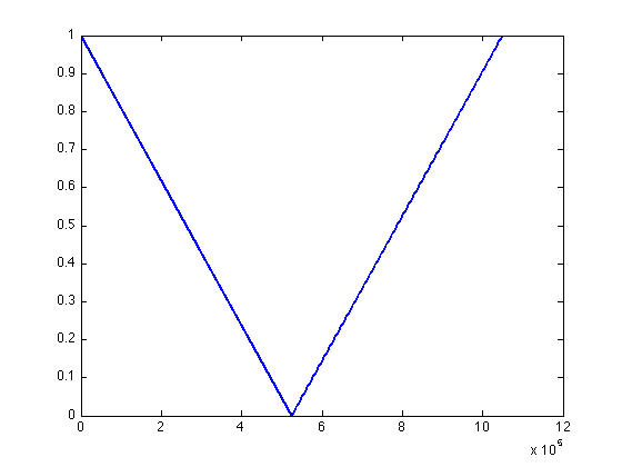
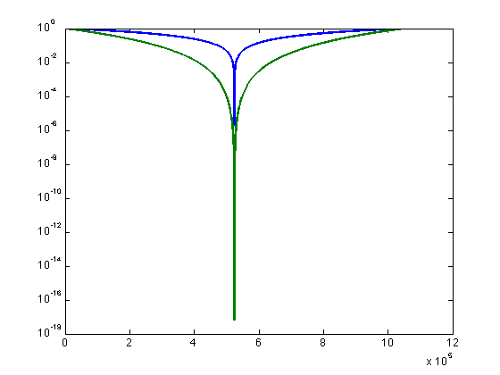
% These are a set of demonstrations to get you comfortable with real-world applications of the
mathematical tools we discussed in class. Although you can copy and paste the MATLAB code directly,
you might want to type it manually.

% We will apply convolution and fourier transforms to two sets of data. The first is a sound
file, on which we will perform frequency space manipulations.

% The builtin MATLAB function, wavread(), allows us to read in sound files in the .wav format.

% Copy the file, ?Something.wav? onto your computer and use the ?cd? command to move to the
directory that has the file. The following command creates a new variable, mySound, whose
contents are the sound file. The length is 1 Mb.

% We will be manipulating this file in frequency space. The builtin function, fft(), takes
the fast fourier transform of the input. There are a few things to note right away: first,
the fft outputs are complex but we can only play real sounds. Second, the plot command may
not do what you might expect if you graph complex numbers. Specifically, it plots the real part
on the x axis and the imaginary parts on the y axis. To manage this, we will use the MATLAB real()
and abs() functions to look at the real part or the magnitudes, sqrt(x2+y2), of the complex numbers. The
imag() function returns the imaginary part, if needed. Finally, the order in which the data are
returned from the fft are a little strange. The first half of the output contains the positive
frequencies from zero to the maximum frequency in the data. The second half of the data are the
negative frequencies (as though we were going backwards in time) arranged from the most negative
to the least. I have suppressed all of this in the exercises.

mySound = wavread('Something.wav');

% Create a new variable, FmyS, containing the fft of the sound file:
FmyS = fft(mySound);

% Create a set of filters. The idea is that we will multiply the fft (or 'spectrum') of the
sound files by a weighting function, or filter. The first filter simply decreases the amplitude
of the high frequencies linearly:
filt1 = abs(-524288:524287)'./524688;

% Another variant decreases the amplitude more rapidly, proportional to s3 (s is the frequency).
filt1sq = filt1.^3;
plot(filt1,'linewidth',2);
hold all
plot(filt1sq ,'linewidth',2);

% The ?holdall? command makes sure that the prior graph is still showing when you add a second.
Make note of the colors of each curve for later. This is how to get MATLAB to form a log plot
along the Y axis:
set(gca, 'YScale', 'log');
Our second filter weights the signal proportional to 1/s:
s = 1:524288;
filt2 = s .^ -1; % This raises each value of s to the -1 power

% Note that because of the curious order of the fft output, we must make a second half for
the negative frequencies. The command, fliplr(), flips right and left in a row vector upside.
The single quote at the end of the command line converts a row vector to a column vector and
vice versa.
filt2 = [filt2, fliplr(filt2)]';
plot(filt2 ,'linewidth',2)
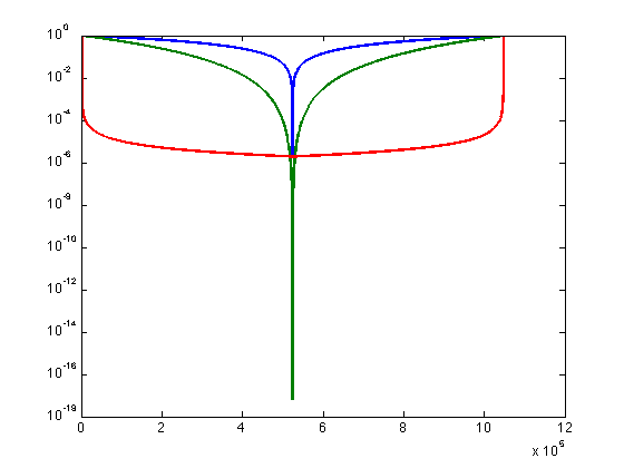
Our final filter is a digital version of what you will be making out of small electronic parts. It has the characteristic that the amplitude is proportional to 1/(1+tau/s):
s = 1:524288;
tau = .0001;
filt3 = 1./(1+s*tau);
filt3 = [filt3, fliplr(filt3)]'; % fliplr is like flipud for row vectors
plot(filt3 ,'linewidth',2);
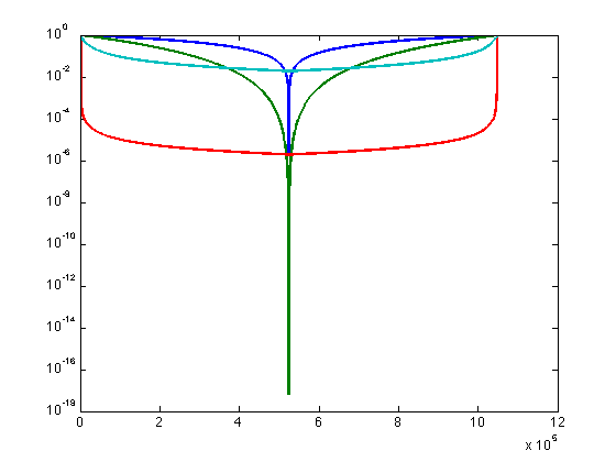
The filters go from 0 to max positive, then from max negative to zero (because of the output order in the fft). It is just
as well to look at only
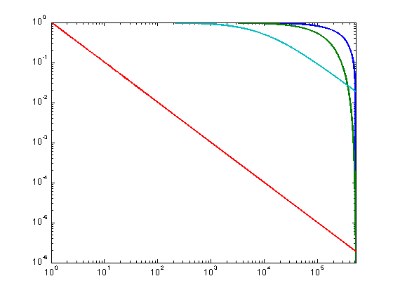
the first half of the filter. Having done so, we can look at these filters with a logarithmic x axis,
which is a little easier to see. The third command
just limits the range on the Y axis:
set(gca,'XLim',[1,524288]);
set(gca, 'XScale', 'log');
set(gca,'YLim',[1e-6 1]);

% Here we apply each of our digital filters by multiplying the Fourier transform of the sound
by the filter weights:
filt1FS   = filt1 .* FmyS;
filt1sqFS = filt1sq .* FmyS;

filt2FS = filt2 .* FmyS;

filt3FS = filt3 .* FmyS;

% To get back from the frequency domain to the time domain, we apply the inverse Fourier transform.
filt1S   = real(ifft(filt1FS));
filt1S   = filt1S / max(filt1S);

filt1sqS = real(ifft(filt1sqFS));
filt1sqS = filt1sqS / max(filt1sqS);

filt2S   = real(ifft(filt2FS));
filt2S   = filt2S / max(filt2S);

filt3S   = real(ifft(filt3FS));
filt3S   = filt3S / max(filt3S);
Compare the results. Can you hear the difference?:
disp('Playing unfiltered sound')
sound(mySound,  44100, 16);
pause(1);

disp('Playing linear filter, filt1')
sound(filt1S,   44100, 16);
pause(1);

disp('Playing squared filter, filt1_sq')
sound(filt1sqS, 44100, 16);
pause(1);

disp('Playing 1/s filter, filt2')
sound(filt2S,   44100, 16);
pause(1);

disp('Playing standard lowpass, filt3')
sound(filt3S,   44100, 16);

% When we started in class we looked at a moving average filter. What does this do to the frequency
characteristics of our signal? The answer may be surprising (unless you followed the in class lecture?)

% An easy way to see this is to use random noise ? containing equal amplitude at all frequencies ? as
an input, then observing the filtered output. We generate noise with the randn() function, then use
the conv() (convolution) function to apply a filter kernel, consisting of the weighted average of 7
consecutive points. Note that:
% 1.	Arguments to the conv() function can be in either order (convolution is commutative)
% 2.	The length of the output from the conv() function is the sum of the lengths of the kernel and input functions.
Playing unfiltered sound
Playing linear filter, filt1
Playing squared filter, filt1_sq
Playing 1/s filter, filt2
Playing standard lowpass, filt3
Filtering by moving average
clf; % create a new figure
N = randn(1, 32768);
kern1 = [1 1 1 1 1 1 1] / 7;
k1StarN = conv(kern1, N);
k1StarN = k1StarN(4:32768+4); % make the output the same length as the input

% The ones() function creates a matrix of ones.
% We could have created kern1 as: kern1 = ones(1,7);
kern2 = ones(1,128) / 128;

k2StarN = conv(kern2, N);
k2StarN = k2StarN(64:(32768+64));
sound(N/max(N),32768);
sound(k1StarN/max(k1StarN),32768);
sound(k2StarN/max(k2StarN),32768);

fN = fft(N);
fk1N = fft(k1StarN);
fk2N = fft(k2StarN);
clf
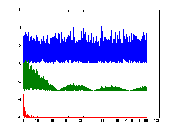
plot(abs(fN(1:16384))/128);
hold all
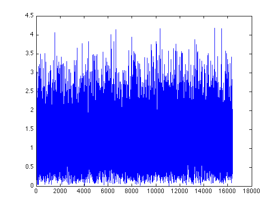
plot(-3+abs(fk1N(1:16384))/128);

plot(-6+abs(fk2N(1:16384))/128);
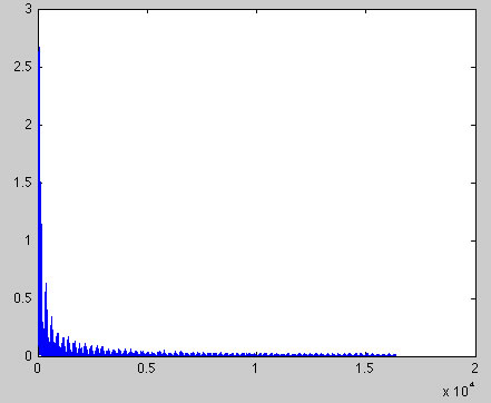
% The plot shows the frequency content after the convolution filter. Notice that some frequencies are suppressed
to zero, whereas others are minimally affected. Longer filters have more prominent weirdness.
Here are some other exercises to think about in order to cement this knowledge: 1. Apply a moving average filter to the Fourier
transform of pure noise,
and observe what happens to its inverse transform (to time domain). What do you expect?
kfN = conv(kern2,fN);
kN = ifft(kfN);
clf
plot(abs(kN(1:16384)));

% 2.	Apply a moving average filter to the frequency domain representations of the sound file and play it back.
kFmyS = conv(kern2,FmyS);
kmyS = real(ifft(kFmyS)); % Turn up the volume to hear this.
sound(kmyS, 44100, 16);

% 3.	Try convolving by sinc, sin(x)/x, functions.  Do you get what you expect?
% 4.	Run the music through a low pass filter
% 5.	Adjust the value of tau for filt3. What happens?