Contents

Linearity: A physicist maxim: Everything is linear to first order

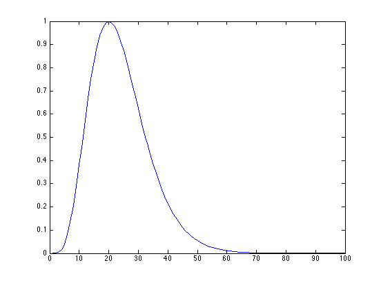
% Consider a very complex and non-linear function:
x = 1:100;
y =(x./20).^5 .* exp(5-(x./4));
% (this is the so-called 'gamma' function)

% Why is this non-linear? Because y(A*x) does not equal A*y(x)

plot(x,y);

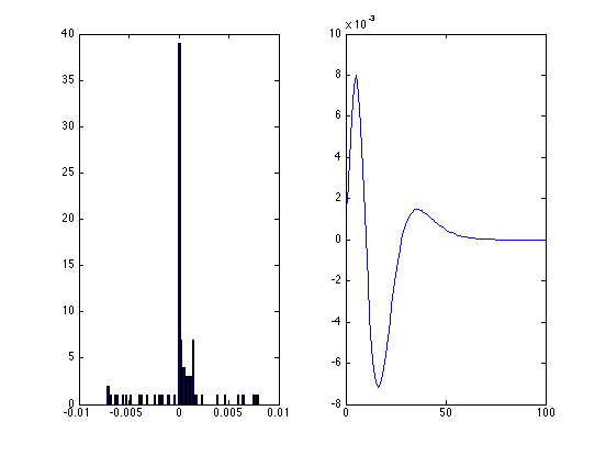
Now consider the local deviations from linearity by looking at groups of 3 consecutive points. The linear approximation locally for the middle point, y(j+1) is y(j) + (y(j+2)-y(j))/2. The error is the difference between that and the actual value of y(j+1)

errors = zeros(1,98);
for j=1:98
    errors(j) = y(j) + (y(j+2)-y(j))/2 - y(j+1);
end;

mean(errors)
std(errors)

subplot(1,2,1)
hist(errors, 100)
subplot(1,2,2)
plot(x(1:98),errors)

ans =

  -4.4157e-06


ans =

    0.0028

The Impulse response

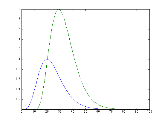
If a system is linear, and its output to a response of area A and duration -> 0 is A(I(t)), then its response to an input of area B at time T will be B(I(t-T) Since we have it here, let's assume that that the initial response looks like our function y

clf;
A = 1;
B = 2;
plot(x,A*y);

hold all;
plot(x(10:100),B*y(1:91));

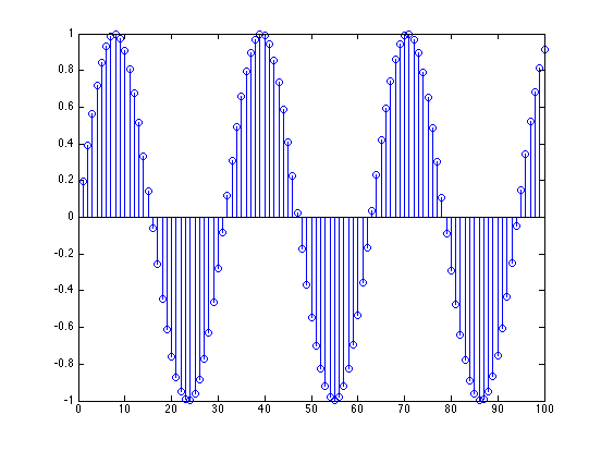
It follows that if we have an input function that is made up piece-wise of discrete values, e.g.

clf;
f = sin(x/5);
stem(x,f)

We can anticipate an output from our function that is made up of the scaled and shifted outputs to each of the discrete inputs

scale_shift = zeros(100,200);
for j=1:100
    scale_shift(j,j:j+99) = f(j) * y;
end

surf(scale_shift)

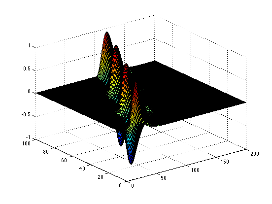
Added together...

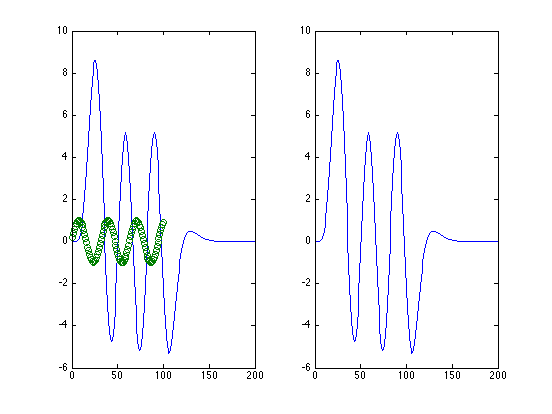
subplot(1,2,1);
output = sum(scale_shift);
plot(output);
hold;
scatter(x,f);

Current plot held

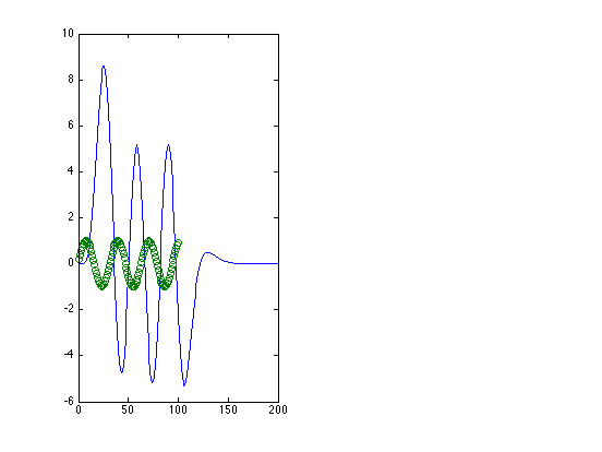
This is the meaning of a convolution. MATLAB has this built in (of course)

subplot(1,2,2)
plot(conv(f,y));

Published with MATLAB® 7.7