Contents
- This simulation shows the convolution theorem in action
- Simulate an amusing signal
- Estimate the response as the convolution of the signal and the impulse response
- Have a look at the Fourier transforms:
- This is the convolution theorem in action.
- Tabulate the errors.
- Consider observing the signal in the presence of small amounts of noise.
- Reapply the convolution theorem to the noisy signal.
- Tabulate the errors.
This simulation shows the convolution theorem in action
First create an impulse response (I am fond of Gamma functions)
clf
clear all;
x=1:1024;
a=5; b=5;
h=(x./(a.*b)).^a .* exp(a-(x./b));
plot(h)

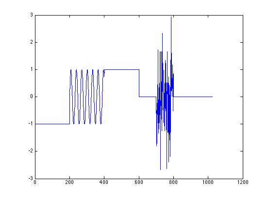
Simulate an amusing signal
clf
x=1:200;
f=[-1 * ones(1,200), sin(x/5),ones(1,200),zeros(1,100),randn(1,100),zeros(1,224)];
plot(f)
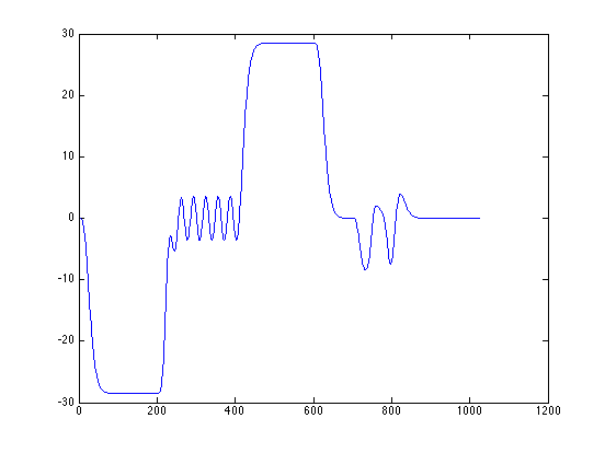
Estimate the response as the convolution of the signal and the impulse response
Notice how the rapidly changing noise signal is highly attenuated. The low frequency (slowly changing) portions pass through, but the abrupt changes from low to high, or high to low, are slowed considerably.
cfh = conv(h,f);
cfh = cfh(1:1024);
plot(cfh)
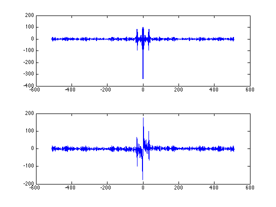
Have a look at the Fourier transforms:
Fh = fft(h);
sFh = fftshift(Fh);
fvals = -512:511;
subplot(2,1,1);
plot(fvals,real(sFh));
subplot(2,1,2);
plot(fvals,imag(sFh));

Ff = fft(f);
sFf = fftshift(Ff);
subplot(2,1,1);
plot(fvals,real(sFf));
subplot(2,1,2);
plot(fvals,imag(sFf));
The convolution, f*h, is equivalent to multiplying the Fourier transforms of f and h Notice in the bottom figure how the high frequency components are attenuated, which helps to explain the result above.
clf
subplot(2,1,1)
plot(fvals,abs(sFf))
subplot(2,1,2)
plot( fvals, abs(sFh .* sFf) );
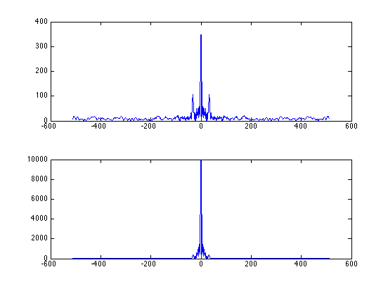
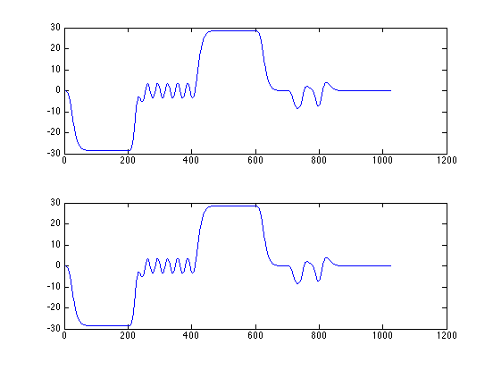
This is the convolution theorem in action.
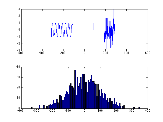
Fcfh = fft(cfh);
deconv = ifft(Fcfh ./ Fh);
subplot(2,1,1)
plot(f);
subplot(2,1,2)
rdeconv = real(deconv);
plot(real(deconv));

Tabulate the errors.
hist(rdeconv - f,100);

Consider observing the signal in the presence of small amounts of noise.
clf
cfhN = cfh + randn(1,1024) * 0.001;
% The top plot shows the original filtered signal.
subplot(2,1,1)
plot(cfh)
% The bottom plot shows the filtered signal with 0.1% added noise, which is
% not detectably different
subplot(2,1,2)
plot(cfhN)
Reapply the convolution theorem to the noisy signal.
FcfhN = fft(cfhN);
deconv = ifft(FcfhN ./ Fh);
% The top plot shows the original signal.
subplot(2,1,1)
plot(fvals,f);
subplot(2,1,2)
% The bottom plot shows the reconstructdd signal with 0.1% added noise
plot(real(deconv));
% Yow! The original signal was completely overwhelmed by even this tiny
% amount of noise.

Tabulate the errors.
hist(real(deconv) - f,100);