Problem Set 3B: Moving to the next dimension

Usually we consider images to have at least two dimension. Fortunately, the analysis tools we have studied can be appied in more than one dimension. In particular, convolution and Fourier transforms are trivially extended into higher dimensions. This is a reflection, in fact, of the linearity of the operations.

A two dimensional Fourier transform is performed on a two dimensional image (or data set) by taking the Fourier transform of each row (or column), and then funding the Fourier transform of each of the resulting columns (or rows).

To do this problem set, you will need to have a copy of the file, 'PS3Bdata.mat' which you can find at:

http://www.brainmapping.org/NITP/PNA/data/PS3Bdata.mat

The following code assumes that you have a copy of the file PS3Bdata.mat in your working directory. To find your working directory, type pwd at the MATLAB command line. Use your computer knowledge to make sure that PS3Bdata.mat is located there.

This problem set uses several new MATLAB commands.
Load in the sample data
Perform the first FFT along the rows
You might find it easier to visually interpret the results after you have performed an fftshift
The 2 dimensional transform is made by taking a second fft along the columns
The fftshift command is so ubiquitous that MATLAB extends it automagically to higher dimensions.
Alternatively, you can look at the magnitude data
Two, three and higher dimension transforms are very common - fftn.
The Fourier transform is completely invertible, though small rounding errors can occur in the digital implementations.
Question 1.
Question 2.

This problem set uses several new MATLAB commands.

To find out more about the command syntax, type: doc command_name at the MATLAB prompt. E.g.,

doc repmat

Load in the sample data

To see what data you have just loaded, use the whos command

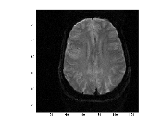
clear all;
load PS3Bdata
whos
clf;
image(TestIm,'CdataMapping','scaled');    % CDataMapping refers to how the data values are converted to grey levels.
axis image;
colormap('gray');   % Present the image in shades of gray

  Name          Size              Bytes  Class     Attributes

  TestIm      128x128            131072  double

Perform the first FFT along the rows

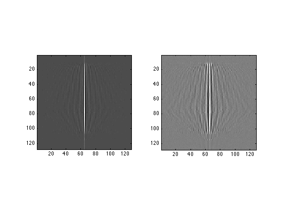
FirstFT = zeros(128,128);
for j=1:128
    FirstFT(j,:) = fft(TestIm(j,:));
end;

subplot(1,2,1)
image(real(FirstFT),'CDataMapping','scaled');
axis image;
subplot(1,2,2)
image(imag(FirstFT),'CDataMapping','scaled');
axis image;

You might find it easier to visually interpret the results after you have performed an fftshift

To learn about the arguments to fftshift, type:

 "doc fftshift"
at the command line.

Each row in the resulting picture is the Fourier transform of a row in the input image.

subplot(1,2,1)
image(real(fftshift(FirstFT,2)),'CDataMapping','scaled');
axis image;
subplot(1,2,2)
image(imag(fftshift(FirstFT,2)),'CDataMapping','scaled');
axis image;

The 2 dimensional transform is made by taking a second fft along the columns

SecondFT = zeros(128,128);
for col=1:128
    SecondFT(:,col) = fft(FirstFT(:,col));
end
subplot(1,2,1)
image(real(SecondFT),'CDataMapping','scaled');
axis image;
subplot(1,2,2)

image(imag(SecondFT),'CDataMapping','scaled');
axis image;

The fftshift command is so ubiquitous that MATLAB extends it automagically to higher dimensions.

This code shows you the 'rings in a puddle' appearance of the typical 2D Fourier transform.

subplot(1,2,1)
image(fftshift(real(SecondFT)),'CDataMapping','scaled');
axis image;
subplot(1,2,2)
image(fftshift(imag(SecondFT)),'CDataMapping','scaled');
axis image;

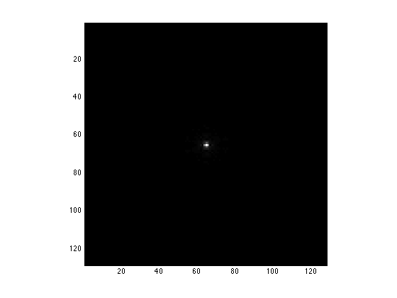
Alternatively, you can look at the magnitude data

clf
image(fftshift(abs(SecondFT)),'CDataMapping','scaled');
axis image;

Two, three and higher dimension transforms are very common - fftn.

MATLAB has a generalized fft command, fftn, to do fft's in higher dimensions. It also has an inverse transform command, ifftn, that does the inverse transform in n-dimensional data.

BackToData = ifftn(SecondFT);
image(abs(BackToData),'CDataMapping','scaled');
axis image;

The Fourier transform is completely invertible, though small rounding errors can occur in the digital implementations.

To show this, make a subtraction. After that, to use the hist command, the data must be made one-dimensional. The MATLAB reshape command does this for you

doc reshape

clf;
hist(reshape(abs(BackToData)-abs(TestIm),1,128*128),100)

Question 1.

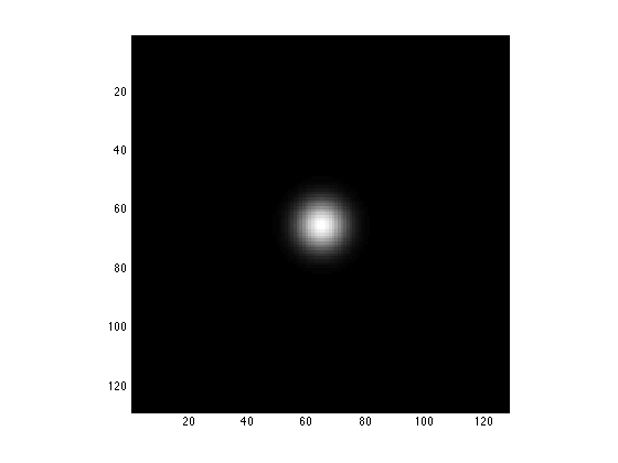
Using your knowledge of the Fourier convolution theorem, make a gaussian-smoothed version of TestIm by multiplying the 2DFT of TestIm by a 2D gausssian. To get you started, here is a 2D gaussian of the same size as the image and its Fourier transform

x=0:127;
g=repmat(exp(-(x-64).^2/64),128,1);
TwoDGauss = g'*g/128;
clear g;
image(abs(TwoDGauss),'CDataMapping','scaled');
axis image;

Question 2.

Make an edge enhanced version of TestIm, by increasing the amplitude of the high spatial frequencies relative to the low. N.B.: HiPassFilter=fftshift(TwoDGauss) would not be a good choice.