
While these notes are somewhat specific to Excel, much of the content pertains to other computer-based Fourier tools.
Fortunately, Excel has some built in functions that make it possible to perform Fourier transforms relatively easily. If you intend to use Excel for this purpose, I encourage you to look through their help files to understand it, but here are a few notes.
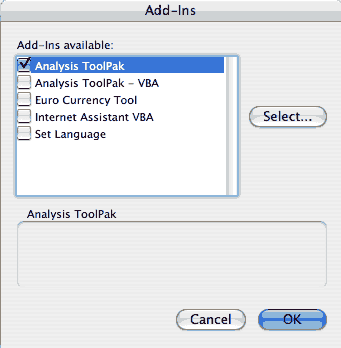
To use the Fourier functions, you must first enable the Analysis ToolPack. From the Tools menu, select "Add-Ins..." then check the Analysis Toolpack and click 'OK'


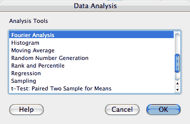
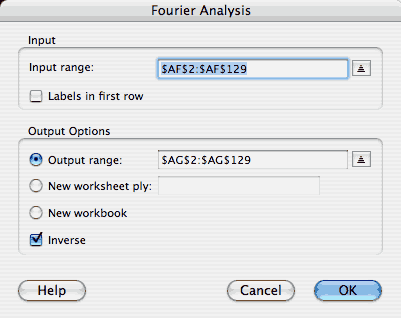
This adds a 'Data Analysis...' item to the Tools menu. If you then select: 'Tools->Data Analysis...' you will get a little list of functions. Select the 'Fourier Analysis' function from that list. Clicking OK brings up the dialog box to control this.


The help file is not too bad from here. You will enter the input numbers into the input range and select a place to put the outputs, and you will select either forward (default) or inverse transform.
The Fourier transform converts a set of numbers into another equal sized set of numbers. However, the computer implementation requires that the size of the set be a power of 2. Thus, you can form the Fourier transform of a set of 128 numbers, but not a set of 100 numbers. If you need to work with non power of 2 sizes, you should pad the ends of the data (usually with zeroes.)
Remember that for real-valued inputs, the transformed data is Hermite symmetric. This means that the positive and negative real parts will be identical, and that the positive and negative imaginary parts will be the same, but of opposite sign. Equivalently, we say that that negative and positive values are complex conjugates of one another. When the Fourier transform completes, the data are in a somewhat odd order. Specifically, the values of positive frequencies are laid out from 0 to the maximum frequency. These are followed by the negative frequency values, which are laid out from the highest to the lowest frequency (-1). The plots I put in the problem set are of the magnitude of the data: sqrt( Real2 + Imaginary2). A complex number and its complex conjugate have the same magnitude. Thus I showed the plots only for positive frequency.
Another quirk of the digital transform is understanding the range of frequencies that appear. If you have 128 points, the transform creates the amplitudes for 64 frequencies - this is a result of what is known as the Nyquist limit, which we will cover later. 0 frequency is represented, however, though there are always an even number of frequencies. This means that the frequency range is asymmetric. If your input is, for example, 16 points long your output frequencies will be in the order:
| 0 | 1/16 | 2/16 | 3/16 | 4/16 | 5/16 | 6/16 | 7/16 | -8/16 | -7/16 | -6/16 | -5/16 | -4/16 | -3/16 | -2/16 | -1/16 |
Meaning that the first cell will be the amplitude at DC (zero frequency), the second will be the amplitude of signals that have a period of one every 16 samples in the input data, etc... If, in this example, you collected a data point every millisecond, the frequencies in Hz would be:
| 0 Hz | 1/16ms = 62.5 Hz | 125 Hz | 187.5Hz | 250 Hz | 312.5 Hz | 375 Hz | 437.5 Hz | -500 Hz | -437.5 Hz | -375 Hz | -312.5 Hz | -250 Hz | -187.5 Hz | -125 Hz | -62.5 Hz |
What is "negative frequency?" Imagine you have a wheel rotating clockwise at 1 rotation/minute. A frequency of -1 rotation/minute would correspond to the wheel turning counter-clockwise at the same rate.
Fourier transforms are operations on complex numbers. In general, the Fourier analysis tool presents its output in Excel's complex number format, which places the complex number in a single cell, with a value such as 123.876 + i546.2. In the table above, each of the cells would contain a complex number. If you need to look at the Real part, you can use the function, IMREAL(). If you need to see the Imaginary part, you call the function IMAGINARY(). To convert to Excel complex format, you use the function, COMPLEX(), which takes two inputs corresponding to the Real and Imaginary parts. For example, if these formulas are entered into the spreadsheet:
|
The resulting values will be: |
|