Contents

MRI Signal to Noise Ratio

Here we explore a little bit about the visibility of images in noise.

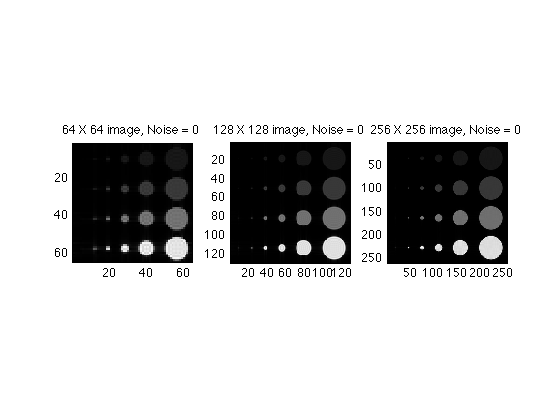
clear;
figure;
set(gcf,'color','white','name','Noise-Free Images');
load imf;   % Loads in a 1024X1024 raw data set;
mygray = [0:1/255:1;0:1/255:1;0:1/255:1]';  % Supplements MATLAB's default 64 level gray scale

imf64 = imf( 512-31:512+32,512-31:512+32 );
imf128 = imf( 512-63:512+64,512-63:512+64 );
imf256 = imf( 512-127:512+128,512-127:512+128 );

subplot(1,3,1)
imagesc(abs(ifftn(fftshift(imf64))));
colormap(mygray);
title('64 X 64 image, Noise = 0');
axis square

subplot(1,3,2)
imagesc(4 * abs(ifftn(fftshift(imf128))));
colormap(mygray);
title('128 X 128 image, Noise = 0');
axis square

subplot(1,3,3)
imagesc(16 * abs(ifftn(fftshift(imf256))));
colormap(mygray);
title('256 X 256 image, Noise = 0');
axis square

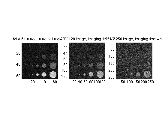
Simulation of minimum imaging time

set(gcf,'color','white','name','Minimum Imaging Time');
subplot(1,3,1)
TheNoise = 8*randn(64,64);
Noisy64 = TheNoise + imf64;
im64 = abs(ifftn(fftshift(Noisy64)));
imagesc(im64);
title('64 X 64 image, Imaging time = 1');
axis square

subplot(1,3,2)
TheNoise = 8*randn(128,128);
Noisy128 = TheNoise + imf128;
imagesc(4*abs(ifftn(fftshift(Noisy128))));
title('128 X 128 image, Imaging time = 2');
axis square

subplot(1,3,3)
TheNoise = 8*randn(256,256);
Noisy256 = TheNoise + imf256;
imagesc(16*abs(ifftn(fftshift(Noisy256))));
title('256 X 256 image, Imaging time = 4');
axis square

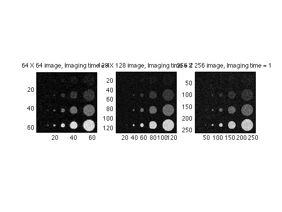
Simulation of constant imaging time

set(gcf,'color','white','name','Constant Imaging Time');
subplot(1,3,1)
imaging_time = 256/64;
TheNoise = 8*randn(64,64) / sqrt(imaging_time);
Noisy64 = TheNoise + imf64;
im64 = abs(ifftn(fftshift(Noisy64)));
imagesc(im64);
title('64 X 64 image, Imaging time = 1');
axis square

subplot(1,3,2)
imaging_time = 128/64;
TheNoise = 8*randn(128,128) / sqrt(imaging_time);
Noisy128 = TheNoise + imf128;
imagesc(4*abs(ifftn(fftshift(Noisy128))));
title('128 X 128 image, Imaging time = 1');
axis square

subplot(1,3,3)
imaging_time = 256/256;
TheNoise = 8*randn(256,256) / sqrt(imaging_time);
Noisy256 = TheNoise + imf256;
imagesc(16*abs(ifftn(fftshift(Noisy256))));
title('256 X 256 image, Imaging time = 1');
axis square

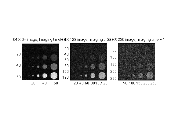
Simulation of constant SNR

set(gcf,'color','white','name','Constant Signal to Noise Ratio');
subplot(1,3,1)
imaging_time = 256/64;
TheNoise = 2*randn(64,64) * sqrt(imaging_time);
Noisy64 = TheNoise + imf64;
im64 = abs(ifftn(fftshift(Noisy64)));
imagesc(im64);
title('64 X 64 image, Imaging time = 4');
axis square

subplot(1,3,2)
imaging_time = 128/64;
TheNoise = 2*randn(128,128) * sqrt(imaging_time);
Noisy128 = TheNoise + imf128;
imagesc(4*abs(ifftn(fftshift(Noisy128))));
title('128 X 128 image, Imaging time = 2');
axis square

subplot(1,3,3)
imaging_time = 256/256;
TheNoise = 2*randn(256,256) * sqrt(imaging_time);
Noisy256 = TheNoise + imf256;
imagesc(16*abs(ifftn(fftshift(Noisy256))));
title('256 X 256 image, Imaging time = 1');
axis square

Published with MATLAB® 7.9