Contents

Properties of K-Space

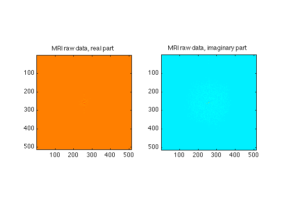
These exercise are intended to give you a sense of the properties of K-space (the MR raw data) and the ways in which the artifacts and behavior of MR images depends on the k-space trajectories and dadta

clear;  % clears data from memory
clf;    % clears the figures
load RawData;   % This is a file containing raw data for a 512 X 512 MR image
whos;   % shows you the characteristics of the input data

mygray = [0:1/255:1;0:1/255:1;0:1/255:1]';  % Supplements MATLAB's default 64 level gray scale

[ydim, xdim] = size(RawData);

% First, let's look at the MR raw data, which has both real and imaginary
% parts.
subplot(1,2,1);
image(real(RawData),'CdataMapping','scaled');
axis square;
set(gcf,'Color','White');
colormap('jet');
title('MRI raw data, real part');

subplot(1,2,2);
image(imag(RawData),'CdataMapping','scaled');
axis square;
title('MRI raw data, imaginary part');

% Note that very little of the signal appears outside of the center regions
% of k=space

  Name           Size               Bytes  Class     Attributes

  RawData      512x512            4194304  double    complex   

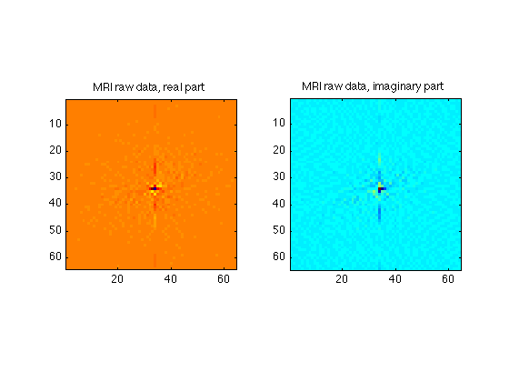
Center of K-Space

We can zoom in on the center 64 X 64 points of k-space to see the data a bit better

Ymid = ydim/2;
Xmid = xdim/2;
Center64 = RawData( Ymid-32:Ymid+31, Xmid-32:Xmid+31 );

subplot(1,2,1);
image(real(Center64),'CdataMapping','scaled');
axis square;
set(gcf,'Color','White');
colormap('jet');
title('MRI raw data, real part');

subplot(1,2,2);
image(imag(Center64),'CdataMapping','scaled');
axis square;
title('MRI raw data, imaginary part');

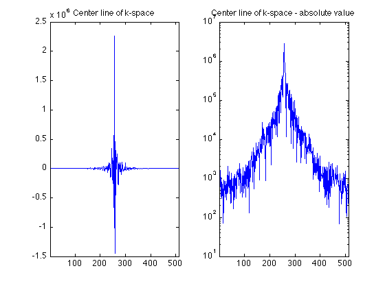
K-space lines

As individual lines, you will see that most look a bit like sinc functions.

clf;
subplot(1,2,1);
plot(real(RawData(256,:)));
set(gca,'xlim',[1 512]);
title('Center line of k-space');
subplot(1,2,2);
plot(abs(RawData(256,:)));
set(gca,'xlim',[1 512]);
set(gca, 'yscale','log');
title('Center line of k-space - absolute value');

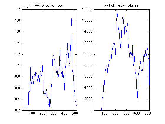
Center projections

The 1D Fourier Transform of the center LINE of K-space is euivalent to the project shadow of the object in the imager along the x axis.

clf;
subplot(1,2,1);
centerProjectionRow = ifft(fftshift(RawData(256,:)));

% The raw data for a REAL object in the scanner generally is complex,
% containing both real and imaginary parts. However, the mechanics of the
% instrument, and effects such as subject motion, actually produce raw data
% result in raw data whose fourier transform is complex. Thus we generally
% look at the magnitude (absolute value) of the images.
plot(abs(centerProjectionRow));
set(gca,'xlim',[1 512]);
title('FFT of center row');

% The 1D Fourier Transform of the center COLUMN of K-space is equivalent to
% the project shadow of the object in the imager along the Y axis.
subplot(1,2,2);
centerProjectionCol = ifft(fftshift(RawData(:,256)));
plot(abs(centerProjectionCol));
set(gca,'xlim',[1 512]);
title('FFT of center column');

The Image is the (inverse) 2DFT of the Raw data

clf;
ReconImage = ifftn(fftshift(RawData));
subplot(1,2,1);

% Note that we generally use the absolute value of the raw data to
% accomodate phase variations from factors such as shim homogeneity.
image(abs(ReconImage), 'CdataMapping','direct');    % I use the direct lookup table so that we can compare intensities
axis image;
colormap(mygray);

% A lower resolution image is formed from the central area of k-space
Center64Image = ifftn(fftshift(Center64));
subplot(1,2,2);
image(abs(Center64Image/64), 'CdataMapping','direct'); % The scaling has to do with integrating a smaller area of k-space
axis image;
title('64X64 matrix');

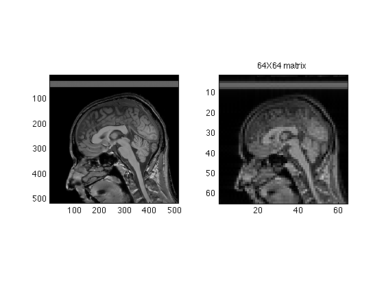
Same idea with Central 128 lines

Center128 = RawData( Ymid-64:Ymid+63, Xmid-64:Xmid+63 );
Center128Image = ifftn(fftshift(Center128));

subplot(1,2,2);
image(abs(Center128Image/16), 'CdataMapping','direct');
axis image;
title('128X128 Matrix');

Images of 512 resolution are rare. We will mostly work with 256x256

Raw256 = RawData( 129:384, 129:384 );   % for later
Center256Image = ifftn(fftshift(Raw256));

subplot(1,2,2);
image(abs(Center256Image/4), 'CdataMapping','direct');
axis image;
title('256x256 Matrix');

remove unused stuff

clear Center64 Center64Image Center128 Center128Image

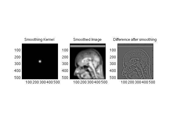
The high k values (periphery of k-space) contain high SPATIAL frequency information.

Attenuating these makes tends to smooth the image. Here, we smoothly attenuate these values by multiplying their intensities by a two dimensional gaussian.

% Create the gaussian:
x=0:511;
SmoothingWidth = 32;
SigmaSquared = (xdim/SmoothingWidth)^2;
g=repmat(exp(-(x-256).^2/SigmaSquared),512,1);
TwoDGauss = g' .* g;

clf;
subplot(1,3,1);
image(abs(TwoDGauss),'CDataMapping','scaled');
title('Smoothing Kernel');
axis image;

% Multiply the k data:
FSmoothRaw = TwoDGauss .* RawData;

% Create a new image
SmoothedRecon = ifftn(fftshift(FSmoothRaw));

subplot(1,3,2);
image(abs(SmoothedRecon), 'CdataMapping','scaled');
title('Smoothed Image');
axis image;

% Plot the difference between the smoothed and original image
subplot(1,3,3);
image(abs(ReconImage) - abs(SmoothedRecon), 'CdataMapping','scaled');
title('Difference after smoothing');
axis image;
% Notice that the difference image is mostly edges

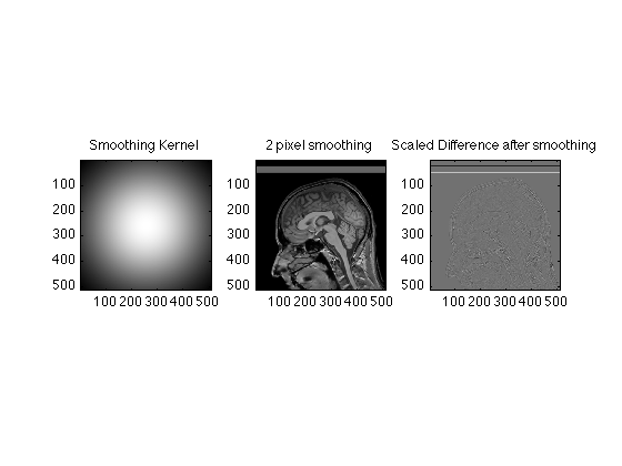
We can smooth less aggressively by making attenuating the high k values less.

SmoothingWidth = 2;
SigmaSquared = (xdim/SmoothingWidth)^2;
g=repmat(exp(-(x-256).^2/SigmaSquared),512,1);
TwoDGauss = g' .* g;

subplot(1,3,1);
image(abs(TwoDGauss),'CDataMapping','scaled');
title('Smoothing Kernel');
axis image;

FSmoothRaw = TwoDGauss .* RawData;
SmoothedRecon = ifftn(fftshift(FSmoothRaw));

subplot(1,3,2);
image(abs(SmoothedRecon), 'CdataMapping','scaled');
title('2 pixel smoothing');
axis image;

subplot(1,3,3);
image(abs(ReconImage) - abs(SmoothedRecon), 'CdataMapping','scaled');
title('Scaled Difference after smoothing');
axis image;
% Here, only the finest details were lost.
% All of these exercises are actually examples of the Fourier convolution
% theorem, by the way. Ask if you want to know more.

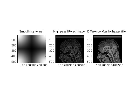
Construct high pass filter

It is just as easy to construct a high pass (edge) filter. Instead of emphasizing the low spatial frequencies we supress them, and use the high spatial frequencies instead.

% We start with a gaussian
SmoothingWidth = 2.5;
SigmaSquared = (xdim/SmoothingWidth)^2;
g=repmat(exp(-(x-256).^2/SigmaSquared),512,1);
TwoDGauss = g' .* g;

% We then use the fftshift command reorder the data
HighPass = fftshift(TwoDGauss);

subplot(1,3,1);
image(abs(HighPass),'CDataMapping','scaled');
title('Smoothing Kernel');
axis image;

FHPRaw = HighPass .* RawData;
HighPassRecon = ifftn(fftshift(FHPRaw));

subplot(1,3,2);
image(abs(HighPassRecon), 'CdataMapping','scaled');
title('High pass filtered image');
axis image;

subplot(1,3,3);
image(abs(ReconImage) - abs(HighPassRecon), 'CdataMapping','direct');
title('Difference after high pass filter');
axis image;


% Exercises
%
% Calculate and show the differences in images acquired with matrix sizes
% of 64X64, 128X128, 256X256 and the original 512X512 image.
%
% Compare the effects of aggressive smoothing on the 512X512 image and the
% 64X64 image.
%
% Explain the presence of a dark line in the spinal cord on the 128X128
% image.
%
% Construct an edge enhanced image

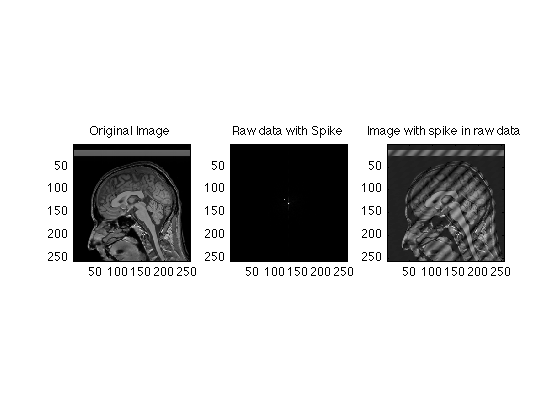
Common artifacts

It is not unusual for a single raw data point to become corrupted from events such as a small static electricity discharge. Here we simulation corruption of a single raw data time point

clear;
mygray = [0:1/255:1;0:1/255:1;0:1/255:1]';  % Supplements MATLAB's default 64 level gray scale

load RawData;
Raw256 = RawData(129:384, 129:384);
clear RawData;
Spike256 = Raw256;
Spike256(120,120) = 1e7;
clf;

subplot(1,3,1);
imagesc(abs(ifftn(fftshift(Raw256))));
colormap(mygray);
title('Original Image');
axis image;

subplot(1,3,2);
imagesc(abs(Spike256));
title('Raw data with Spike');
axis image;

subplot(1,3,3);
imagesc(abs(ifftn(fftshift(Spike256))));
title('Image with spike in raw data');
axis image;

% Because the images are rectified (absolute value) spikes contaminate the
% whole image

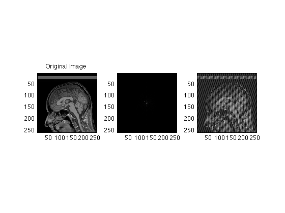
Two or more spikes creates a sort of herringbone pattern

Spike256(130,150) = 1e7;
subplot(1,3,2);
imagesc((abs(Spike256)));
axis image;

subplot(1,3,3);
imagesc(abs(ifftn(Spike256)));
axis image;

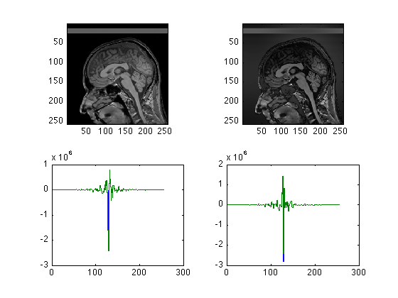
Saturation

clear Spike256;
% Like all electronic devices, the MRI scanner has certain hardware
% limitations. If, for example, the input levels are too high, the input
% amplifiers will "clip". This can and does happen when the pre-scan is not
% completed properly.

% We can simulate this easily by setting a maximum signal intensity
% threshold lower than the actual signal amplitude
clf;
subplot(2,2,1);
imagesc(abs(ifftn(fftshift(Raw256))));
axis image;

Clip = reshape( Raw256, 256*256,1 ); % convert to a linear vector for convenience;
MaxReal = max(abs(real(Clip)));    % Find the maxima separately in the real and imaginary parts
MaxImag = max(abs(imag(Clip)));
DataMax = max( MaxReal, MaxImag);

Thresh = 0.2 * DataMax; % Set the threshold to 50% of the actual value

count = 0;
R=0;
I=0;
for pt = 1:size(Clip)
    rpt = real(Clip(pt));
    ipt = imag(Clip(pt));
    if( abs(rpt)> Thresh || abs(ipt)>Thresh)
        if abs(rpt) > Thresh
            R = abs(Thresh/rpt) * rpt;
            count = count+1;
        end
        if abs(ipt) > Thresh
            I = abs(Thresh/ipt) * ipt;
            count = count+1;
        end
        Clip(pt) = R + 1i*I;
    end
end

Clip = reshape(Clip, 256, 256); % Back to square raw data

subplot(2,2,2);
imagesc(abs(ifftn(Clip)));
axis image;

subplot(2,2,3);
stairs(1:256,real(Raw256(130,:)));
hold all;
stairs(1:256,real(Clip(130,:)));

subplot(2,2,4);
stairs(1:256,imag(Raw256(130,:)));
hold all;
stairs(1:256,imag(Clip(130,:)));

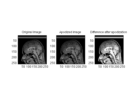
Apodization.

This section simulates, crudely, the effect of T2 star signal decay during readout.

clear;
clf;

load RawData;
mygray = [0:1/255:1;0:1/255:1;0:1/255:1]';  % Supplements MATLAB's default 64 level gray scale


% we will work here with the more conventional 256 X 256 images
[ydim, xdim] = size(RawData);
Ymid = ydim/2;
Xmid = ydim/2;
RawData = RawData(129:384, 129:384)/4;  % again, the factor fo 4 intensity scaling comes from the smaller than original matrix size.
[ydim, xdim] = size(RawData);
Ymid = ydim/2;
Xmid = ydim/2;
ReconImage = ifftn(fftshift(RawData));

ReadoutDuration = 16;   % msec
T2star = 50;    % msec
Samples = (0:xdim-1) * ReadoutDuration / (T2star * (xdim-1)) ;
Apodizer = exp(-Samples);
Time = 0:ReadoutDuration/(xdim-1):ReadoutDuration;
clf;
plot(Time,Apodizer);
set(gca,'ylim',[0 1]);
title('T2 decay during readout');

pause(5)
% Apply the weighting to each line of the original data.
ApodizedData = repmat(Apodizer,ydim,1) .* RawData;
ApodizedImage = ifftn(fftshift(ApodizedData));

subplot(1,3,1);
image( abs(ReconImage), 'CdataMapping','direct' );
axis image;
title('Original Image');

subplot(1,3,2);
image(abs(ApodizedImage), 'CdataMapping','direct');
colormap(mygray);
axis image;
title('Apodized image');

subplot(1,3,3);
image( abs(ReconImage - abs(ApodizedImage)), 'CdataMapping','direct' );
title('Difference after apodization');
axis image;

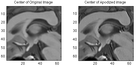
More aggressive apodization happens in long readout scans such as EPI

ReadoutDuration = 128;   % msec
T2star = 32;    % msec
Samples = (0:xdim-1) * ReadoutDuration / (T2star * (xdim-1)) ;
Apodizer = exp(-Samples);
Time = 0:ReadoutDuration/(xdim-1):ReadoutDuration;
clf;
plot(Time,Apodizer);
set(gca,'ylim',[0 1]);
title('T2 decay during readout');

pause(5);
ApodizedData = repmat(Apodizer,ydim,1) .* RawData;
ApodizedImage = ifftn(fftshift(ApodizedData));

subplot(1,3,1);
image(abs(ReconImage), 'CdataMapping','scaled');
colormap(mygray);
title('Original Image');
axis image;

subplot(1,3,2);
image( abs(ApodizedImage), 'CdataMapping','scaled' );
title('Apodized image');
axis image;

subplot(1,3,3);
image( abs(ReconImage - abs(ApodizedImage)), 'CdataMapping','direct' );
title('Difference after apodization');
axis image;

% Here is a zoomed view
pause(5)
clf;
subplot(1,2,1);
imagesc(abs(ReconImage(Ymid-32:Ymid+31, Xmid-32:Ymid+31)));
title('Center of Original Image');
axis image;

subplot(1,2,2);
imagesc(abs(ApodizedImage(Ymid-32:Ymid+31, Xmid-32:Ymid+31)));
title('Center of Apodized image');
axis image;

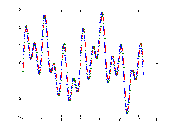
Fourier Shift theorem

t = 0:pi/64:4*pi-pi/64;
s1 = sin(t);
s3 = sin(3.3*t);
s5 = sin(2*pi*t);
s = s1+s3+s5;
Fs = fft(s);

a = .002*pi;
S = -127:128;
m = exp(-2*pi*1i*S*a);
shifted = m .* fftshift(Fs);
shiftedSignal = ifft(fftshift(shifted));
clf;
pause(1);
plot(t,(s),'.');
hold;
plot(t,(s));
hold all;
plot(t,(shiftedSignal),'.');
plot(t,(shiftedSignal));

Current plot held
Warning: Imaginary parts of complex X and/or Y
arguments ignored 
Warning: Imaginary parts of complex X and/or Y
arguments ignored 

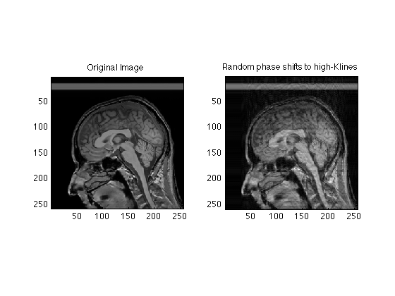
Motion artifact simulation

clf;
clear;

% The following initializes the randomization each time
RandStream.setDefaultStream(RandStream('mt19937ar','seed',sum(100*clock)));

mygray = [0:1/255:1;0:1/255:1;0:1/255:1]';
load RawData;
Raw256 = RawData(128:384, 129:384);% work with a 256 x 256 image

subplot(1,2,1);
imagesc(abs(ifftn(fftshift(Raw256)))); axis square; colormap(mygray);  % a single line for convenience in cut and paste
title('Original Image');

[ys xs] = size(Raw256);

C = Raw256;

% we will corrupt the phases slightly
for line = 1:ys;
    shift = exp(1i*0.5*randn());    % adds a random phase shift to the lines
    C(line,:) = Raw256(line,:) * shift;
end
subplot(1,2,2);
imagesc(abs(ifftn(fftshift(C))));
title('Random phase shift');
axis square;
colormap(mygray);
disp('Click on Image');
waitforbuttonpress;

C = Raw256;

% we will corrupt a few lines near the center of k-space
for line = 120:138;
    shift = exp(1i*0.5*randn());    % adds a random phase shift to the middle lines
    C(line,:) = Raw256(line,:) * shift;
end
subplot(1,2,2);
imagesc(abs(ifftn(fftshift(C))));
title('Random phase shifts to middle lines');
axis square;
colormap(mygray);

disp('Click on Image');
waitforbuttonpress;
C = Raw256;

% we will corrupt a few lines
for line = [64:90, 146:168]
    shift = exp(1i*3*randn());    % adds a random phase shift to the middle lines
    C(line,:) = Raw256(line,:) * shift;
end
subplot(1,2,2);
imagesc(abs(ifftn(fftshift(C))));
title('Random phase shifts to high-Klines');
axis square;
colormap(mygray);

Click on Image
Click on Image

Published with MATLAB® 7.9