Echo-planar imaging (EPI) and functional MRI
Mark S. Cohen, Ph.D.
To appear in Bandettini and Moonen: Functional MRI
©1998 PA Bandettini and C Moonen. For academic use only.
Contents
- Introduction
- What is EPI?
- SNR
- Bandwidth and Artifacts
- Resolution
- Hardware Requirements
- dB/dt and Safety and Head Gradients
- Contrast Variants
- Volume EPI
- Conclusions
- References
1. Introduction
Since the first days of human NMR imaging, reaching back to the late 1970’s [1-3] (and others), imaging time has presented a serious practical limitation. The practical reality of ordinary structural imaging is that normal subjects are willing to tolerate perhaps an hour of lying inside of the imaging magnet, and are able to stay still for little more than fifteen minutes. Both NMR contrast and signal to noise ratio, however, are time-dependent phenomena. As a result, imaging time and image quality have traditionally been at odds for all manner of magnetic resonance imaging. Figure 1 shows the relationship between imaging time and a variety of interesting biological phenomena. Figure 1B, conceived by Van J. Wedeen at Harvard University, shows the steady decrease in practical MR imaging times that took place over the first decade of human imaging and demonstrates the remarkably steady logarithmic improvements in imaging speed that have characterized the field. It is perhaps even more remarkable, therefore, that today’s fastest practical imaging method, echo-planar imaging, or EPI, was conceived in 1977 [4], before the veritable explosion in clinical use of MRI. EPI achieved largely novelty status however, until it found a driving application – namely functional MR imaging and especially functional neuroimaging. A major factor in the relatively slow acceptance of EPI is that it is just plain hard to implement as we will see below.
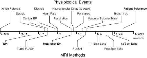
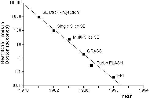
Figure 1A. Comparison of physiological processes and imaging speeds of common magnetic resonance imaging methods. To avoid image artifacts, scan times must not be longer than the duration of motion. To study the dynamics of these processes, the imaging times must be substantially shorter. EPI and multi-shot EPI, the methods discussed in this chapter, are indicated in bold. B. Fastest MRI scan times in Boston (after Van Wedeen) as a function of year and technology. |
2. What is EPI?
While MRI as conventionally practiced builds up the data for an image from a series of discrete signal samples, EPI is a method to form a complete image from a single data sample, or a single "shot". The speed advantages can be astonishing. For example, a typical T2-weighted imaging series (to form an image whose contrast depends predominantly on the intrinsic tissue magnetization parameter, T2) requires that the time between excitation pulses, known as "TR" be two to three times longer than the intrinsic tissue magnetization parameter, T1. The T1 of biological samples is typically on the order of a second or so (cerebrospinal fluid, or CSF, can have much longer T1’s of several seconds); TR must therefore be 3 seconds or more. A more or less typical MR image is formed from 128 repeated samples, so that the imaging time for our canonical T2 weighted scan is about 384 seconds, or more than 6.5 minutes. By comparison, the EPI approach collects all of the image data, for an image of the same resolution, in 40 to 150 milliseconds (depending on hardware and contrast considerations). This reflects a nearly 10,000-fold speed gain.
Although, as we will discuss below, there are myriad variations, EPI is fundamentally just a trick of spatial encoding. To understand the difference between EPI and conventional imaging, it is necessary therefore, to have some understanding of spatial encoding in MRI.
2.1 MRI Spatial Encoding
Tomographic image formation requires spatial encoding in three dimensions. In most cases, one dimension is determined by slice selective excitation [5] (refer to Figure 2 for axis labels). Briefly, a radio frequency excitation pulse with a narrow frequency range is transmitted to the subject in the presence of a spatial magnetic field gradient. Because the magnetic resonance phenomenon depends on an exact match between the radio frequency excitation pulse frequency and the proton spin frequency, which depends in turn, on the local magnetic field, this pulse will excite the MR signal over a correspondingly narrow range of locations: an imaging slice. The differences between EPI and conventional imaging occur in the remaining "in-plane" spatial encoding.
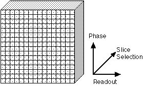
Figure 2. The three axes used for spatial encoding of MR images. One dimension of spatial encoding is achieved by slice selective excitation (the "Slice Selection" axis). The other two are encoded by phase and frequency. Some texts will refer to the Slice Selection axis as the "Z" axis. The Readout axis is variously labeled the "Frequency" or "X" axis; the Phase Encoding axis is sometimes labeled the "Y" axis. |
When a magnetic field gradient is applied across this excited slice, it will cause the spin frequency to be a function of position. The pixel size, or spatial resolution, of an MR image depends on the product (actually the integral) of the imaging gradient amplitudes and their ON duration. Specifically, the pixel size is equal to 1/gGt, where g is the Larmor constant (4258 Hz/gauss), G is the gradient amplitude, usually expressed in gauss/cm, and t is the gradient on time. A gradient of 0.5 gauss/cm, left on for 10 msec, for example, yields a spatial resolution of 0.47 mm. This, however, reflects spatial encoding along one in-plane dimension only – the "Readout" direction. In ordinary two-dimensional Fourier transform imaging, the encoding for the second in-plane dimension is created by applying a brief gradient pulse (along a second gradient axis) before each readout line. For 128 lines of resolution in this axis, 128 separate lines must be acquired, each for 10 msec. The total readout duration is therefore 128 x 10 msec, or 1.28 seconds. Unfortunately, the MR signal lasts for only about 100 milliseconds (limited by T2) and over the course of a 1.28 second readout duration (spatial encoding period) the signal will have decayed to nothing.
In EPI, much larger gradient amplitudes are used. A gradient of about 2.5 gauss/cm is typical, but human imagers with gradient amplitudes in excess of 5 gauss/cm are achievable. With five times the gradient amplitude, the encoding duration can be reduced by five-fold, to 2 msec/line, so that the total spatial encoding time for our reference image is reduced from 1.28 seconds to 256 msec. The human brain has a T2 of about 100 msec at typical imaging field strengths. Thus, a 256 msec readout might be marginally realistic. In practice, however, for reasons discussed below, this is not a practical configuration. Most significantly, the gradients cannot instantly reach such large magnitudes, and the rise time therefore becomes a significant fraction of the readout duration. Secondly, the decay of the MR signal during readout introduces blurring into the images [6]. Because of these tradeoffs, most EPI studies are performed at somewhat lower resolution. In-plane voxel sizes between 1.5 and 3 mm are typical.
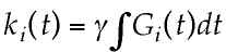
In many cases all of this is somewhat easier to understand in terms of "k-space", where k-space is a representation of the MRI raw data before it has been Fourier-transformed in order to make an image [7-10]. The signal location in k-space is the integral of the gradient amplitude and on-time:
 ,
,
where ki is the location in k-space along the i axis, Gi(t) is the gradient amplitude along the i axis as a function of time, g is the Larmor constant, and t is the gradient on-time. As the gradient-time product increases, that is, as the signal is encoded to higher k values, the image resolution increases. Thus, in order to make an MR image of any desired final resolution, we must collect MR data over a corresponding area of k-space.
In conventional MRI, k-space is covered line by line, as suggested in figure 3A. Following each RF excitation, a single line of raw data is collected along kx (the readout axis), with sequential lines acquired at different displacement along the ky axis. Because a separate excitation step is required prior to the collection of each data line, the total imaging time depends on the time between excitations (also known as tr) as well as on the total number of data lines collected. The latter depend on the desired resolution and field of view in the final images.
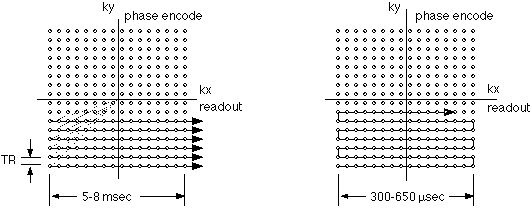
Figure 3A and 3B. K-space traversal patterns used in conventional imaging (A. left) and echo-planar imaging (B. right). Small circles represent the required data samples. In conventional imaging, each raw data line is separately acquired after an RF excitation. As a result, tr elapses between the collection of each data line. In EPI, the lines are acquired continuously, in a raster-like pattern, with as little as 300 µsec elapsing from line to line.
Figure 3B shows the k-space trajectory used in echo-planar imaging. Here, the sequential raw data lines are acquired immediately after one another. In modern imagers, the collection of each data line can be as rapid as 300 microseconds. Figure 4 shows the gradient encoding scheme needed for the EPI k-space trajectory. The rapid back and forth traversal of the readout axis is preformed by using an oscillating readout gradient. Following each readout excursion, a brief pulse of the phase encoding gradient is used to move to the next line in the phase encode direction. |
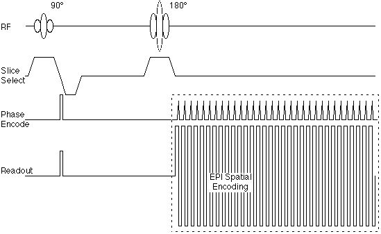
Figure 4. Echo-planar pulse sequence corresponding to the k-space trajectory shown in figure 3B. |
Figure 4 suggests also that the echo-planar encoding portion of the sequence can be encapsulated as a module that is somewhat independent of the radio frequency pulse sequence. As we will see below, this is important, as the image contrast is determined largely by the RF sequence, rather than the gradient spatial encoding.
3. SNR
Signal to Noise ratio (SNR) in MRI is a function of:
- Available transverse magnetization (pulse sequence and contrast)
- Imaging time (or more precisely, time spent receiving the signal)
- Bandwidth – the signal sampling rate
- Field Strength
- RF coil loading, coupling and sensitivity.
- Voxel volume
Echo planar imaging carries the advantage (by contrast with the so-called gradient echo methods such as FLASH, GRASS, etc…[11]) that the full magnetization is available as signal: In a single shot method, all of the longitudinal magnetization may be used in image formation without a penalty in overall imaging time. The imaging time consideration also works to the advantage of EPI: in a typical EPI sequence, as used in ƒMRI, signal may be collected for well over 75% of the imaging time, leading to a very high efficiency. EPI pays a penalty in bandwidth, however. The imaging speed in EPI comes from the use of very high amplitude field gradients which, in turn allow, and require, very rapid sampling. While conventional MR imaging may use receiver bandwidths up to about 32 kHz, bandwidths of 300 kHz are typical in EPI and drop the usable SNR by about two-thirds. Field strength, and RF coil considerations are not pulse-sequence dependent. All told, theoretical analyses and direct measurement have demonstrated a nearly five-fold SNR advantage of EPI over FLASH studies [12] for comparable voxel volume.
4. Bandwidth and Artifacts
The bandwidth of an MR image refers the difference in MR frequencies between adjacent pixels, as well as to the total range of frequencies that make up an image. In conventional imaging , the bandwidth, per pixel, is ordinarily kept comparable to the chemical shift between fat and water. In a 1.5 Tesla instrument, for example, a pixel bandwidth of 125 Hz is typical (the fat-water shift is about 220 Hz). In this case, the fat and water components of a single voxel will be shifted from one another by about 1 pixel, which is an acceptable imaging artifact. At first blush, one would expect that the pixel bandwidth in EPI would be very high, due to the rapid sampling rate. This is, in fact, true along the readout axis. The continuous encoding scheme used in EPI, however, results in a relatively low bandwidth along the phase encoding axis; 30 Hz/pixel is typical. This causes several difficult artifacts to occur in EPI.
4.1 Chemical Shift
In echo planar imaging, the very low bandwidth along the phase encode axis results in substantial chemical shift artifacts. At 1.5 Tesla, for example, using a 30 Hz/pixel bandwidth, fat and water are displaced by about 8 pixels. Further, the voxel sizes in EPI are usually rather large, for the reasons discussed above. Using a more or less typical 3 mm voxel, fat and water may be displaced from one another by 2.5 cm. This problems scales with field strength, so that in a 3 Tesla scanner the fat water chemical shift approaches 5 cm. Since most body tissues contain at least some water and fat, it is absolutely necessary to correct for the chemical shift problems.
Fortunately, there are a number of good technologies to manage chemical shift [13]. In the vast majority of cases, only the water component of the MR signal is of clinical interest. This is always the case in functional neuroimaging, where the lipid content of the brain is very low and the dominant source of fat signal is the component found in skin. It is therefore reasonable to simply suppress the fat signal outright. Usually, this is done by applying a fat saturation pulse prior to imaging. Because the chemical shift between fat and water is quite large, one can transmit a 90° pulse at the fat frequency without significantly affecting the water signal. After this pulse the fat signal will be in the transverse plane and it can be dephased easily by applying a gradient pulse. Until the fat signal has had time enough to recover its longitudinal magnetization it will not appear in the images. This so-called chemical shift saturation method does require excellent magnetic field homogeneity so that the frequencies of fat and water are well-resolved. Fortunately, today’s imaging instruments easily meet this requirement.
An alternative method of suppression is to use STIR (short TI inversion recovery)[14]. This approach takes advantage of the T1 difference between fat and other body tissues. An inversion (180°) pulse is applied immediately prior to the EPI imaging sequence timed such that the magnetization of fat is recovering through zero at the time of the 90° excitation pulse. Because the fat has no magnetization at that time, the 90° pulse does not result in the formation of any signal from fat. While STIR is a very effective method of fat suppression, it has side effects that make it less desirable. First of all, it alters the contrast of the images overall, as it adds T1 contrast. Secondly, the method works best if the inversion pulse is applied only when the tissue is fully magnetized. The latter requires that inversion recovery be used only with long TR images.
4.2 Shape Distortion
The low bandwidth of EPI causes a much less manageable artifact in shape distortion. Even in a well-shimmed magnet, the human head will magnetize unevenly so that the MR frequency may differ from point to point by about 1 part per million (ppm). These small frequency differences result in spatial displacement of the signal in the resulting images. Most investigators simply tolerate the typical one or two pixel distortion as an acceptable artifact. Generally, however, this artifact is correctable. It is possible to measure the magnetic field in the head and then to apply a correction to the MR image to shift the signal to its correct location [15].
The shape distortions are a frequent cause of concern in functional neuroimaging, as it is often desirable to superimpose regions of brain activation onto higher resolution structural images, that are usually acquired conventionally (e.g., with a much higher bandwidth). In this case, the activation maps will not be registered properly with the structural data set.
4.3 Ghosting
When the MR field gradients are switched on and off, the time varying magnetic field of the gradients results in current induction (eddy currents) in the various conducting surfaces of the rest of the imaging instrument. These, in turn, set up magnetic field gradients that may persist after the primary gradients are switched off. Such eddy currents are a problem in both conventional and echo-planar imaging, but are more severe in EPI. The gradient amplitudes, and particularly the gradient switching rates, used in EPI are much greater and induce larger eddy currents. Further, the long readout period in EPI results in more opportunity for image distortion from eddy currents.
A particularly common EPI artifact is so-called "ghosting" from eddy currents. This results from the time-dependent frequency shift created by the time-dependent eddy currents. Because of the back and forth trajectory in k-space used in EPI (see figure 3), the frequency shifts create a phase difference from line to line in the raw data. When the data are Fourier transformed, the phase shift creates a phase ambiguity in the images, such that part of the signal appears 90° out of phase, or one half image away. This ghosting structure is frequently referred to as an "N/2 ghost". Figure 5 shows schematically the appearance of such a ghost image.
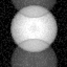
Figure 5. Appearance of a so-called N/2 ghost that occurs frequently in echo-planar imaging. Such "ghosts" are the result of small line-by-line phase errors that can take place during spatial encoding. |
The correction of image ghosts may take several forms. Probably the most robust scheme is to design the gradient coils critically such that eddy current induction is minimized. At present the most effective method is to use shielded or "screened" gradient coils, in which a separate set of gradient coils is counterwound around outside the primary coil set to cancel any external magnetic fields. Because gradient efficiency drops as the fifth power of the radius, even a small gap between primary and secondary gradients allows for a non-zero gradient inside the coil and a zero gradient outside [16].
Elimination of the N/2 ghost also requires critical calibration of the timing between signal digitization and gradient activity. Delays of a few microseconds result in line-by-line phase discrepancies because of the alternating left-right trajectory along the readout axis in k-space (figure 3). These errors can be tuned out in hardware by adjusting the sampling clock, and may be adjusted further in software by adding an appropriate phase shift to the raw data. The latter can be performed by an exponential multiplication. An alternative approach to ghost correction is to acquire a reference scan in the absence of phase encoding and to use this as a basis for determination of the time-dependent phase shifts [17,18].
5. Resolution
Resolution, or voxel size, depends on the maximum gradient amplitude-time product in the raw data. Increases in resolution require either increases in gradient amplitude, increases in gradient duration, or both. Neither is easy to come by. As we will see below, the power requirements for the gradients in EPI can be quite large [19,20]. Further, switching to gradients rapidly to very high amplitudes may ultimately result in unacceptable safety problems. Increasing the duration of the gradient pulses lowers the effective image bandwidth and increases the sensitivity of the images to shape distortion and other artifacts. At this writing, the highest performance body gradient sets reach amplitudes of up to 3.6 gauss/cm with a rise time of 179 µsec using a sinusoidal waveform. This results in a 3 mm pixel size in the readout axis [21].
Fortunately, a variety of k-space encoding schemes are available to improve spatial resolution. Increases in resolution along the phase encoding axis are available simply by extending the total duration of the echo planar readout (box shown in dotted lines in figure 4) [12]. This increases the total displacement along the ky (phase encoding k axis) at the cost of a decrease in bandwidth and an increase in minimum echo time. Doubling the encoding period, for example, will reduce the pixel size and the bandwidth, per pixel, by a factor of two. Shape distortions from field inhomogeneity will remain constant in distance (as expressed in millimeters), though they will cover double the number of pixels. This tradeoff frequently works well.
A useful way to increase resolution along the readout axis results from the Hermitian symmetry property of k-space [22,23]. Formally, reflections about the axes in k-space are complex conjugates; a data point at (kx, ky) is equal to the complex conjugate of the data point at (-kx, ky) or at (kx, -ky). This symmetry property implies that it is necessary to acquire only half of the entire MR raw data space to form a complete MR image. A very efficient way to achieve high resolution in a single shot EPI experiment is to use a long readout duration along ky and to acquire only the positive (or negative) values in kx. Prior to image formation, it is a relatively simple matter to calculate the data that make up the uncollected portion of the image and then to Fourier transform the entire raw data set to form a complete image (figure 6A).
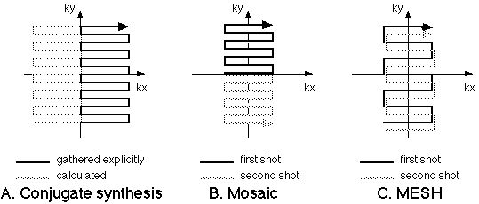
Figure 6. Resolution enhancement approaches for EPI. A. The conjugate synthesis method (variously called Half-Fourier, Half-NEX or partial-k) takes advantage of the conjugate symmetry of k-spaceso that only half of the raw data need be collected to form a complete MR image. The Mosaic method (B) collects regions of k-spacein tiles. C. In MESH, the k-spaceregions are collected in interleaved fashion, usually with a higher amplitude phase encoding step. |
The complex conjugation "trick" outlined above requires a few pre-conditions to work properly. First, it depends on the desired image having no "imaginary" component. What this means in practice, is that the user must not be interested in any phase deviations along the image. Such phase difference might result, for example, from local field inhomogeneities or motion and are usually of little concern to the researcher in functional neuroimaging. Secondly, any phase variations in the image must be relatively small; otherwise, the reconstruction will result in ghost-like artifacts from locations with large phase shifts. Finally, the raw data must be well-centered in k-space for the reflection property to be accurate. Similarly to the process of eddy current correction discussed above, this requirement is achieved by a combination of hardware and software engineering. Figure 7 shows example images, each collected in a single shot, using the conjugate synthesis approach. The in-plane resolution is about 1.5 mm.
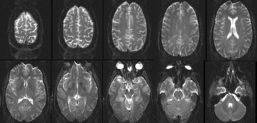
Figure 7. Single-shot EPI images of the human head with 1.5 mm in-plane resolution and 3 mm slice thickness, collected using the conjugate synthesis method. |
While true EPI is a single shot experiment (that is, a single excitation pulse results in a complete image), a variety of EPI hybrids, using multiple excitations per image, may be used to increase spatial resolution. The two most often used include the MESH and Mosaic methods [24]. In the Mosaic method, figure 6B, each excitation is used to cover a different region of k-space and the resulting data are tiled together to form an image of any desired resolution. The MESH technique is slightly subtler. Here, a larger phase encoding step is used so that data collected from separate RF excitations may be interleaved. The important result in MESH imaging is a wider bandwidth in the final image, which may be desirable in reducing imaging artifacts. The multi-shot hybrids have a signal to noise ratio advantage as well: SNR increases with the square root of the acquisition time, so that the SNR is about 40% better in the two shot than in the single shot scans. The multiple shot and conjugate synthesis methods can be combined over a wide range of variations to produce echo-planar images of very high resolution [12].
EPI resolution is limited, ultimately, by the SNR of the images. Since typical EPI data are collected over 40 to 50 msec or so, as compared to the nearly 1 second of acquisition time spent on a conventional scan, the SNR is down by a factor of more than 4-fold at comparable resolution on this basis alone. As shown in figure 7, single shot images with voxel volumes of 3 x 1.5 x 1.5 mm (= 6.75mm3) offer acceptable SNR at 3 Tesla. In fact, the measured SNR differences between conventional and EPI data in human subjects are much less than predicted on the basis of theory. This is likely due to the fact that tiny motions in the conventional imaging set result in an overall increase in apparent image noise. At the present time, it seems that EPI spatial resolution is largely gradient limited.
6. Hardware Requirements
EPI is a demanding sequence for the imaging instrument. Good quality images require high performance gradients with rapid rise times, high peak amplitudes, high accuracy and low eddy currents. The demands on the data acquisition system are considerable as well. Because the data are sampled so rapidly, very fast analog to digital converters (ADC’s), up to 2 MHz, are required. The ADC subsystems, however, are becoming more widely available due to advances in semiconductor technology.
6.1 Gradient Power
A typical body gradient coil in an MR system will have an efficiency of about 1 gauss/cm per 100 amps. Thus, a current of 250 to 350 amps is required to produce acceptably high gradient amplitudes for EPI. Further, the inductance of the typical body coil is about 1 milliHenry. The gradient slew rate (the rate of rise) is determined by the rate of change in current (di/dt). This is calculated easily. For example, to achieve a 200 µsec rise time to 3.5 gauss/cm requires that di/dt equal 350 amps/175 µsec, or 2 x 10⁶ amps/second. With a coil inductance, L, of 1 mH, the required driving voltage is:
V = Ldi/dt = 2000 Volts.
A conventional power system would need to deliver 2000 Volts at 350 amps, or 750,000 Watts to meet this requirement. Most EPI-capable amplifier systems therefore use some form of non-linear amplification using either inductive or capacitive energy storage devices. These implementations recognize that it is generally not necessary to simultaneously source both high current and high voltage to the highly reactive gradient load.
The required accuracy of the gradient waveforms adds another complicating factor. Any deviations from the ideal waveform could result in phase errors in the images. Such deviations can results from eddy currents, physical instabilities or amplifier distortion. One efficient way to manage this problem is to synchronize the signal digitization to the integral of the measured gradient activity, such that the data are sampled uniformly in k-space
7. dB/dt and Safety and Head Gradients
It has been recognized since the early days of MRI that the rapidly switched magnetic field gradients in imaging instruments result in current induction in the patients. The pioneering work of Reilly [25-27], based on direct modeling using the Hodgkin and Huxley equations for neuronal excitability, suggested operational margins below which gradient switching rate (dB/dt) was not likely to be a cause of concern. At that time, gradient switching rates above the predicted neural firing threshold were not practical to achieve. Once the non-linear amplifier methods became feasible, however, it became possible to routinely exceed the threshold of sensation using imaging gradients [28-31]. Most of the present day imaging systems have gradient performance that is limited to just below the typical threshold of sensory stimulation.
There is an alternative, however. The induced current in the patient is proportional not only to the rate of change of the magnetic field, but also to the cross-sectional area of the body exposed to the changing field. For example, it is now well-known that the sensory threshold is higher for gradients that switch along the sagittal axis than for those that switch along the coronal axis, because the cross sectional area of the typical supine person is much larger in the coronal than in the sagittal plane. Further, the maximum dB/dt occurs at the ends of the imaging coil, where the magnetic fields are at their maximum. A shorter coil, therefore, will have a reduced dB/dt. Probably the best solution in functional neuroimaging is to build head-only gradient coils. Such a devices gains safety/sensory threshold margins due both to their reduced length and to the reduced cross-sectional area over which the gradients occur. The cross sectional area of the human neck is less than one-sixth that of the chest. The gradient coil length can be reduced by a factor of at least 2, and probably more than three. Therefore the stimulation threshold, in terms of imaging gradient switching, will be reduced by at least ten, and probably more than 20-fold.
Shorter and smaller gradients offer another set of advantages: the gradient efficiency scales with fifth power of the radius, so that reduced the diameter two-fold can increase the gradient strength by a factor of 32. Thus, the smaller gradients not only enable the use of larger amplitudes with good safety margins, but also make such strong gradients practical to implement. At this writing, the major equipment manufacturers have expressed little interest in special purpose head gradients. In the end, however, it is likely the market will demand such tools for high-performance functional neuroimaging.
8. Contrast Variants
Because EPI is fundamentally just a spatial encoding scheme, there are already a wide variety of variants that can be used to offer a correspondingly wide range of contrast behaviors.
8.1 Spin Echo
Figure 4 shows the most common implementation of EPI as used for clinical imaging: the spin echo sequence. Here the spatial encoding "module" is preceded by a 90° excitation pulse and a 180° echo-forming pulse, resulting in the formation of a Hahn echo [32] during the readout period. Such images have signal intensity (SI) that is well described by the equation:
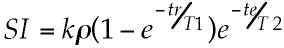 ,
,
where k represents sequence independent factors such as magnetic field strength and RF coil sensitivity, r is the tissue proton density, tr is the repetition time and te is the "echo time" or the time from the excitation pulse to the center of the readout period. Such images show relatively little sensitivity to local field inhomogeneities (at least as they relate to contrast) and behave similarly to conventional MR images. A key difference, however, is that in a single shot EPI study, the tr is effectively infinite, so that the images are obtained with little or no T1 contrast. This is a decided advantage in clinical T2-weighted studies where the T1 and T2 contrast mechanisms when manifest simultaneously, tend to result in an overall reduction in image contrast.
8.2 Gradient Echo
The first practical rapid imaging method was arguably the FLASH (fast low angle shot) sequence developed by Frahm and Haase [11] that has spawned a large number of variants known collectively as "gradient echo" techniques. The name refers to the fact that in these sequences, the 180° echo-forming pulse is omitted, and the signal is refocused solely by the gradients. EPI versions of the FLASH scans are possible and are the most commonly used method for functional neuroimaging today. Figure 8 shows the generalized "gradient echo" EPI sequence.

Figure 8. Gradient Echo EPI sequence. In this sequence, the EPI data collection follows a single RF pulse, whose flip angle, a, is adjusted to set up the preferred contrast. |
The gradient echo EPI sequence is used for several reasons. First, and perhaps most importantly for functional imaging, the contrast behavior includes a T2*, as opposed to a T2 component. That is, the signal intensity decays after excitation at a rate determined by local field inhomogeneities. As described in other sections of this book, it is thought that the dominant mechanism in so-called BOLD functional imaging is the increased decay rate of the MR signal in the presence of field inhomogeneities produced by deoxyhemoglobin. Thus, an imaging sequence sensitive to such local variations is ideal. In gradient echo EPI it is possible also to use shorter TR’s without suffering large signal losses, as the smaller excitation flip angle results in less disturbance from magnetic equilibrium and therefore shorter relaxation recovery times. Gradient echo EPI at frame rates of up to 16 frames/second has been used to produce good quality real-time images of the human heart during the normal contractile cycle [12]. For non-spin echo scans it is possible to calculate the "Ernst" angle, a, at which the signal will be maximal for any combination of tr and T1 [33]:
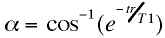 .
.
Since the ordinary functional imaging application is to acquire a series of EPI scans at a non-infinite tr, the gradient echo methods can confer a slight signal advantage over spin echo studies. This advantage increases at shorter tr.
8.3 Offset Spin Echo
By adjusting the relative timing of the Hahn spin echo and the EPI readout module, it is possible to offset the RF echo from the center of k-space. It is by now well-known that the contrast in MR images is dominated by the signal contrast that occurs at the center of k-space, as this region of the raw data encodes the largest spatial features of the images. In the offset spin echo method, varying degrees of susceptibility-related contrast are incorporated into the images. This method has been suggested as an approach to modulating somewhat independently the signal loss from large and small field perturbers [34] and as a method for directly measuring line broadening [35]. In the limit, as the Hahn echo is delayed to beyond the EPI readout, the offset spin echo scan becomes identical to the gradient echo scan. The offset spin echo method may have increasingly important applications at higher magnetic field strengths where the inherent functional imaging contrast is greater in BOLD studies and the artifacts from non-ideal magnetic become more severe. Figure 9 shows the offset spin echo sequence.

Figure 9. Offset spin echo EPI sequence. The offset refers to the relative timing of the spin echo formed by the 90°-180° pulse pair and the center of the EPI readout period, which ordinarily is the center of k-space. |
8.4 Inversion Preparation
As discussed in the context of fat suppression, the addition of a 180° inversion pulse prior to the standard spin echo EPI sequence results in an inversion recovery EPI scan. Such images have easily controlled T1 contrast according to the equation
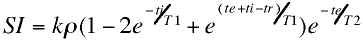
where ti is the time between the inversion and excitation pulses. The inversion recovery EPI sequence is shown in figure 10.
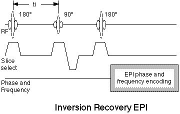
Figure 10. Inversion recovery EPI pulse sequence. The addition of a 180° RF pulse at a time, ti, before the standard spin echo EPI scan results in inversion-recovery contrast behavior. |
The inversion recovery method and its several variants have been used to produced water-suppressed images, similar to the FLAIR method used conventionally and have proven useful in the measurement of blood flow and perfusion.
9. Volume EPI
EPI as typically practiced is a two-dimensional encoding strategy. In most cases, as suggested above, the third dimension is provided by selective excitation. An alternative is to use phase encoding in the slice selection direction to create a 3D volume image [36,37], as shown in figure 11.
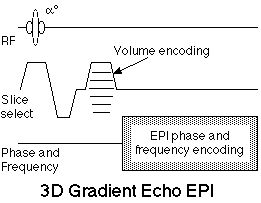
Figure 11. 3D, or Volume echo-planar scan. This is a multi-shot EPI hybrid, where an additional phase encoding step is applied along the slice selection axis with each excitation. After 3D Fourier transformation, these data yield a contiguous multi-slice image set. The sequence is shown using gradient echo contrast, though a 180° echo-forming pulse can be added for spin echo contrast. |
Volume EPI has theoretical advantages in SNR. Because the same volume is repeatedly sampled, albeit with different phase encoding, the signal to noise ratio scales with the square root of the number of phase encodes, effectively the number of slices. Thus a 32 slice data set will have nearly six fold higher SNR than a comparable single slice data set. Using a similar volume sequence, it is possible to collect, for example a sixteen slice volume study of the human heart in only 400 msec [38]. This approach should be highly efficient in functional neuroimaging as well, where contiguous multi-slice image sets are highly desirable. The tr used in the sequence must be reduced by a factor equal to the number of slices to yield the same sampling density. Thus, to acquire an image every 3.2 msec as part of a 32 slice volume, a tr of 100 msec is required. For this reason, shallow flip angle, FLASH-type, imaging is used so that the scanning can be performed at the tissue Ernst angle.
This differs signficantly from so-called echo-volumnar imaging (EVI) in which the entire volume is collected following a single excitation pulse [39]. As of this writing, EVI is not entirely practical because the extended total readout required greatly exceeds the T2*’s of most tissues at clinical field strengths.
10. Conclusions
Echo-planar imaging is at this time the fastest and most flexible approach to MR imaging, offering considerable freedom in the selection of contrast and resolution parameters. It is, however, a technologically challenging method that requires that the imaging system operate at near its performance limits in gradient amplitude and rise times, system stability, and overall noise figure. Further, EPI can suffer from serious artifacts in shape distortion and image ghosts that require extra attention from the researcher. All told, however, the decided advantages of EPI in functional neuroimaging have placed it very much in demand for fMRI applications and have served to drive the technology development both in the academic research laboratory and with major commercial vendors, essentially all of whom now offer EPI products.
Notwithstanding the considerable efforts that have gone into EPI, there are still major advances to be gained. Chief among them will be the practical performance gains that can be achieved with ultra-high performance local gradient coils, which will improve image quality by reducing shape distortions and other bandwidth-related artifacts, while increasing the comfortable operating margin that avoids sensory stimulation.
With the relatively recent dissemination of product level EPI hardware into consumer sites, the future of EPI is rosy indeed and will continue to be driven by the increasingly important clinical applications of functional neuroimaging.
References
- Mansfield, P., I.L. Pykett, and P.G. Morris. Human whole body line-scan imaging by NMR. Br J Radiol. 51(611):921-2. 1978.
- Damadian, R., M. Goldsmith, and L. Minkoff. NMR in cancer, FONAR image of the live human body. Physiol. Chem. Phys. 9:97-. 1977.
- Pykett, I.L. and P. Mansfield. A line scan image study of a tumorous rat leg by NMR. Phys Med Biol. 23(5):961-7. 1978.
- Mansfield, P. Multi-planar image formation using NMR spin echoes. J Phys C. 10:L55-L58. 1977.
- Mansfield, P. and A.A. Maudsley. Medical imaging by NMR. Br J Radiol. 50(591):188-94. 1977.
- Farzaneh, F., S.J. Riederer, and N.J. Pelc. Analysis of T2 limitations and off-resonance effects on spatial resolution and artifacts in echo-planar imaging. Magn Reson Med. 14(1):123-39. 1990.
- Twieg, D. The k-trajectory formulation of the NMR imaging process with applications in analysis and synthesis of imaging methods. Medical Physics. 10(5):610-621. 1983.
- Twieg, D. Acquisition and accuracy in rapid NMR imaging methods. Magnetic Resonance in Medicine. 2:437-452. 1985.
- Ljunggren, S. A simple graphical representation of Fourier-based imaging methods. Journal of Magnetic Resonance. 54:338-343. 1983.
- Brown, T., B. Kincaid, and K. Ugurbil. NMR chemical shift imaging in three dimensions. Proceedings of the National Academy of Science. 79:3532. 1982.
- Frahm, J., A. Haase, and D. Matthaei. Rapid NMR imaging of dynamic processes using the FLASH technique. Magn Reson Med. 3(2):321-7. 1986.
- Cohen, M.S. and R.M. Weisskoff. Ultra-fast imaging. Magn Reson Imaging. 9(1):1-37. 1991.
- Weisskoff, R., M.S. Cohen, and R. Rzedzian. Fat suppression techniques: a comparison of results in instant imaging. in Society for Magnetic Resonance in Medicine. abstr. 836. 1989.
- Bydder, G. and I. Young. MR imaging: clinical use of the inversion recovery sequence. Journal of Computer Assisted Tomography. 9(4):659-675. 1985.
- Jezzard, P. and R.S. Balaban. Correction for Geometric Distortion in Echo Planar Images from Bo Field Variations. Magnetic Resonance in Medicine. 34(1):65-73. 1995.
- Turner, R. and R.M. Bowley. Passive screening of switched magnetic field gradients. Journal of Physics E (Scientific Instruments). vol.19,(no.10):876-9. 1986.
- Bruder, H., H. Fischer, F. Schmitt, and H.-E. Reinfelder. Reconstruction procedures for Echo Planar Imaging. in Society for Magnetic Resonance in Medicine. abstr. 359. 1989.
- Schmitt, F., H. Fischer, and G. Görtler. Useful filterings and phase corrections for EPI derived from a calibration scan. in Society for Magnetic Resonance Imaging, works in progress. abstr. 464. 1990.
- Dickinson, R., F. Goldie, and D. Firmin. Gradient power requirements for echo-planar imaging. in Society for Magnetic Resonance in Medicine. abstr. 828. 1989.
- Rohan, M. Practical limits to gradient coil design. in Society of Magnetic Resonance in Medicine. abstr. 963. 1989.
- Cohen, M.S., D.A. Kelley, M.L. Rohan, and P.A. Roemer. An MR instrument optimized for intracranial neuroimaging. in Human Brain Mapping 96. abstr. P1A1-007. 1996.
- Margosian, P. Faster MR imaging - imaging with half the data. in Society for Magnetic Resonance in Medicine. abstr. 1024. 1985.
- Rzedzian, R. Method of high speed imaging with improved spatial resolution using partial k-space acquisitions1988, US patent:
- Rzedzian, R. High speed, high resolution, spin echo imaging by Mosaic scan and MESH. in Society for Magnetic Resonance in Medicine. abstr. 51. 1987.
- Reilly, J. Peripheral nerve stimulation by induced electric currents: exposure to time-varying magnetic fields. Medical & Biological Engineering and Computing. 27:101-110. 1989.
- Reilly, J. Cardiac sensitivity to electrical stimulation1989, Metatec Associates:
- Reilly, J. Peripheral nerve stimulation and cardiac excitation by time-varying magnetic fields: a comparison of thresholds1990, The Office of Science and Technology Center for Devices and Radiological Health; US Food and Drug Administration:
- Cohen, M.S., R.M. Weisskoff, R.R. Rzedzian, and H.L. Kantor. Sensory stimulation by time-varying magnetic fields. Magn Reson Med. 14(2):409-14. 1990.
- Budinger, T.F., H. Fischer, D. Hentschel, H.E. Reinfelder, and F. Schmitt. Physiological effects of fast oscillating magnetic field gradients. J Comput Assist Tomogr. 15(6):909-14. 1991.
- Rohan, M. and R. Rzedzian. Stimulation by time-varying magnetic fields. in preparation. 1992.
- Bourland, J., G. Mouchawar, J. Nyehuis, L. Geddes, K. Foster, J. Jones, and G. Graber. Transchest magnetic (eddy-current) stimulation of the dog heart. Medical and Biological Engineering and Computing. 28:196-198. 1990.
- Hahn, E. Spin echoes. Physical Review. 80(4):580-594. 1950.
- Ernst, R. and W. Anderson. Application of Fourier transform spectroscopy to magnetic resonance. Reviews of Scientific Instruments. 37:93-102. 1966.
- Baker, J., M.S. Cohen, C. Stern, K. Kwong, J. Belliveau, and B. Rosen. The effect of slice thickness and echo time on the detection of signal change during echo-planar functional imaging. in Society of Magnetic Resonance in Medicine 11th Annual Meeting. abstr. 1822. 1992.
- Hoppel, B.E., J.R. Baker, R.M. Weisskoff, and B.R. Rosen. The dynamic response of DR2 and DR2' during photic activation. in Society of Magnetic Resonance in Medicine. abstr. 1993.
- Cohen, M.S., R. Weisskoff, and H. Kantor. Evidence of peripheral stimulation by time-varying magnetic fields. in Radiological Society of North America. abstr. 382. 1989.
- Cohen, M.S. and M. Rohan. 3D volume imaging with Instant Scan. in Society for Magnetic Resonance in Medicine. abstr. 831. 1989.
- Cohen, M.S., R. Weisskoff, M. Rohan, and T. Brady. 400 msec volume imaging of the heart. in Tenth Annual Meeting of the Society of Magnetic Resonance in Medicine. abstr. 840. 1991.
- Harvey, P. and P. Mansfield. Advances in echo-volumar imaging (EVI). in European Congress of Radiology? abstr. 111. 1990.