 |
| This manuscript is copyrighted to Raven Press and is not to be copied or distributed without express permission of the publisher. It appears in web-served form only to serve the educational purposes of the author. |
Magnetic Resonance Imaging (MRI) always involves a complex balance of final signal to noise ratio (SNR) against a host of user-specified parameters such as resolution, contrast, scan time, field of view and the like. The total available nuclear magnetic resonance signal in biological tissues is extremely small, a problem aggravated by the typical needs of the researcher or clinician for contrast and resolution. Improvements in spatial resolution, for example, necessitate dividing that limited quantity of signal into ever smaller chunks or voxels; improvements in contrast ordinarily are made by selectively diminishing the signal from some tissues while attempting to retain signal from others.
In magnetic resonance imaging (MRI) as currently practiced (we will call this "conventional" as distinct from "echo-planar" imaging) this challenge is addressed by sampling the signal repeatedly, and building up an image data set gradually from these repeated samples. Simply stated, Echo-planar imaging (EPI) demands the formation of a complete image following a single excitatory pulse, collecting the complete data set in the short time that the free induction nuclear magnetic resonance (NMR) signal is still detectable, e.g., in a time limited by T2*.
In practice, EPI places enormous demands on the imaging hardware and on the creativity of the physicist and engineers constructing system hardware and software, and the specific technologies used to answer to these demands form much of the text of the present manuscript. In this chapter, we will consider some of the principles of MR imaging with field gradients and will try to place EPI in this context.
The nuclei of many atoms, most typically hydrogen, behave as though they are spinning about an axis. The motion of these positively charged particles results in the creation of a magnetic field. When such a particle is placed into a static magnetic field (usually known as "B0") its angular momentum results in precession of the nuclear spin about the B0 field. The precessional frequency (f) is a simple function of the magnitude of B0,
f = gB0, (1)
where, for protons, g = 42.58 MHz/Tesla. In other words, in a one Tesla magnetic field, the hydrogen nuclei (protons) will precess about the axis of the applied field at a rate of about 42 million cycles per second. The precessional motion of these tiny nuclear magnets can be observed by the current they induce in any nearby conductor or antenna. It is this set of fundamental principles that forms the physical basis of both nuclear magnetic resonance spectroscopy and imaging.
Once the MR signal has been created, it is necessary to spatially encode it in order to form an image: one must develop a means to determine the strength of the signal as a function of position. The method for doing this is based upon the realization that creating a spatially variant (inhomogeneous) magnetic field will cause the signal frequency to vary with position (per equation 1). In the simplest case, the magnetic field (and therefore the MR frequency) will be a linear function of position:
B0 = Gx + K = f/g (2)
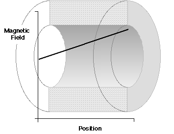
where G is the magnitude of a "gradient" field, x is the position in space, and k is a constant field onto which that gradient is imposed (figure 1). When a gradient is applied, the strength of the MR signal at each frequency will give a measure of the signal strength at each position.
|
| Figure 1. Electromagnetic gradient coils are used to impose a spatially variant magnetic field within a large homogeneous magnetic field. The graph (black) shows the resulting magnetic field as a function of position within the static magnet (grey). |
With larger gradient field amplitudes, the frequency differences between adjacent spins are increased; it is thus possible to resolve smaller differences in position and thereby to improve the spatial resolution of the images. The key to observing the frequency differences is to sample the MR signal during the time that the gradients are applied.
What is needed, then, is a means for determining the signal strength as a function of frequency. Fortunately, that tool was provided to us some 170 years ago and is known as the "Fourier transform" (FT) after its creator, Joseph Fourier. He showed that any signal could be generated by combining a possibly infinite series of sine waves at different frequencies, and showed further how to determine those frequencies and their amplitudes. While this chapter will not attempt to deal analytically with the FT, we will refer to it and its properties from time to time. For a more complete picture, the reader is directed to any of a number of texts on the topic, such as Bracewell's, "The Fourier Transform and its Applications" [1].
Generally, we must localize the MR signal in three dimensions. Currently, for most MR imaging, one dimension of localization is performed using slice selective excitation [2] ; the remaining two-dimensional localization is performed using field gradients as described above. To explain how the latter is done, we will first explore the manner in which the MR signal evolves while a gradient is turned on, and then introduce the concept of "k-space" as a description of the MR raw data. With that background, it is a relatively straightforward task to understand the many variants of EPI.
After the initial RF excitation, or during the spin echo, the magnetization from protons everywhere throughout the sample will be precessing in-phase and, to the extent that the magnetic field is homogeneous and uniform, these protons will be precessing at the same frequency. In imaging, as mentioned above, gradients are used to convert position to frequency. Once such gradients are turned on, the protons along the gradient axis will begin to precess at different frequencies, and will thus begin to de-phase (along axes perpendicular to the gradients the spins will be at the same frequency. A collection of spins at the same frequency is referred to as a spin isochromat). So, one effect of the gradients is to cause a position-dependent phase shift.
 |
| Figure 2. Spin Isochromats. A spin isochromat refers to a collection of nuclear spins precessing at the same frequency. In the presence of magnetic field gradients, spins along a line perpendicular to the gradients will be arranged in isochromats. Continued application of the gradients will result in a phase dispersion between isochromats. The phase differences increase as long as the gradients are applied. The figure on the left represents the phase dispersion after a brief period of t seconds, while the figure on the right shows the accumulated phase difference after 2t seconds. |
Clearly, since frequency is a temporal phenomenon, it is not possible to detect it instantaneously. Less obvious is the fact that the so-called "discrete Fourier transform" (the digital version of the FT) can differentiate the locations of isochromats with one-full cycle (360°) of phase difference. This impacts directly the achievable spatial resolution.
Consider an example: Suppose that we are able to produce a magnetic field gradient of 10-3 Tesla/meter (1 gauss/cm). This will cause spins one centimeter apart to differ in frequency by about 4,258 Hertz (from equation 1). If that gradient is left on for 1/4,258 seconds (about 0.25 msec) then spins one centimeter apart will differ in phase by 360° and can thus be detected as different in position by the Fourier transform. To achieve millimeter resolution, the gradients will need to be left on for ten times as long (2.5 msec), or run at ten times the amplitude (10 gauss/cm). It is the product of the gradient amplitude, and its duration, that determines the final resolution. It also follows that if the gradients are left on for only a very brief period, there will be very little net spatial encoding; the resulting images would have very poor spatial resolution and would differentiate only the largest features of the images. In general then, as the gradient-time product increases, the phase difference between spins in different positions increases, and we are able to detect smaller differences in position through the Fourier transform.
Recognizing that the gradient-time product determines the spatial resolution, we are ready to introduce the concept of "k-space." Note that the MR signals will be collected in the presence of field gradients. If we were to plot the received MR signal starting at the moment that the gradients are switched on, we would see that the data accumulate features about smaller and smaller features of the images (as the gradient-time product increases). This would be a graph of k-space where the horizontal, or "k" axis is the cumulative gradient-time product. Clearly the larger k values will refer to finer image details (i.e., higher spatial frequency).
Because the gradient amplitudes may vary with time, we generally look at the integral of the gradient-time product to get a sense of the amount of spatial encoding that has occurred:
ki = gGidt
(3)
where the subscript "i" indicates that the gradient is applied along the "i" axis.
To develop intuition about the 2-dimensional case consider that:
Figure 3 presents the concepts in statements 1) and 2) graphically. As the data are sampled at discrete points in time (in the process of analog to digital conversion) the phase evolution of the signal depends on the history of the signal prior to each sample point. To the extent that the gradients alter the signal, small gradient amplitudes for long durations are equivalent to large gradient amplitudes for short durations. When the gradients are turned off, and the field is uniform, the signal (or at least its spatial encoding) remains constant.
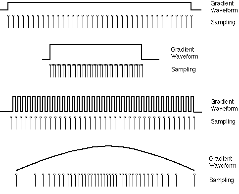 |
| Figure 3. The MR signal is sampled digitally in the presence of magnetic field gradients that cause the precessional frequency of the protons to vary as a function of position. Each digital sample will represent a single data point in the raw data (k) space As the signal is sampled discretely, rather than continuously, the spatial encoding depends only on the integral of the gradient waveform, rather than its shape. Thus, the four spatial encoding schemes sketched above all perform identical spatial encoding. In the first, a modest gradient amplitude is used with regularly spaced samples in time, to produce equally spaced samples in k-space. In the second scheme, application of a larger gradient amplitude allows the use of more rapid sampling. In the third scheme, the gradients are pulsed at high amplitude between successive points. This is analogous to the approach used for "phase" encoding in conventional imaging. the final scheme shows the use of a time-varying gradient waveform. By appropriately adjusting the sample points in time, it becomes possible to space the data samples evenly in k-space in the final data. The amplitude of the gradient determines the rate at which k-space is traversed. |
In conventional imaging, we take advantage of this by applying a gradient along one axis (the "readout" or "frequency-encoding" axis) during signal acquisition, which in typical clinical instruments lasts for five to ten milliseconds. The gradient along the second axis (the "phase-encoding" axis) is applied briefly, immediately prior to readout. Adjacent points along each of the two axes are ordinarily separated by the same "k" distance. However, the time that passes between collection of adjacent points in the two directions can be much different. For the conventional imaging schemes, the time between adjacent points along the phase encode axis is equal to "TR," because the signal, whose T2 is often only slightly longer than the nominal 5 to 10 milliseconds readout period, must be re-formed in the time between the collection of each readout line.
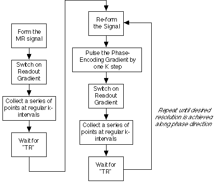 |
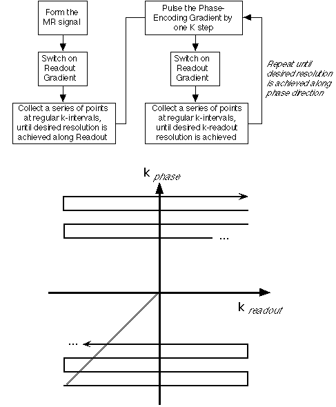
| Figure 4. Flow chart of the gradient encoding scheme for conventional imaging. After the initial formation of the MR signal, a readout gradient is turned on, causing it to be encoded in the readout direction, that is to move along the k-readout direction. Each time the gradient-time product has reached a desired increment, the data are sampled, until a sufficient total displacement has occurred to achieve the desired spatial resolution along that axis. By this time the MR signal will generally have decayed to the point that it needs to be re-formed, either through another excitation, or in the case of RARE or Fast Spin Echo imaging, by an additional echo-forming 180° pulse.
At this point, the phase-encoding gradient is pulsed briefly, displacing the signal in the k-phase direction and the readout process is repeated. The excitation - phase encode - readout cycle is repeated until the desired net displacement in the phase encode direction is achieved. |
Using standard gradient and digitization hardware it ordinarily takes about 3 milliseconds to encode the MR signal, in one dimension, to 1 mm resolution. In order to form the final image, we require the data at every combination of phase and frequency encoding and we, therefore, must repeat the readout encoding once for each k-step in the phase direction. To acquire 64 such readout lines, each at a different displacement along the k-phase direction, would therefore require at least 64x3 msec, or nearly 200 msec. Since this is far longer than the T2 of typical body tissues, this is not a practical readout period. It is for this reason that the pulsed phase-encoding gradient scheme outlined above is used, since it ensures adequate MR signal during the entire data encoding and collection period.
Consider how this might appear in a map of k-space. During the time that gradients are applied, the signal makes a trajectory to a new position, corresponding to a new gradient-time product, in a direction determined by the magnitude of the gradients (the vector sum of any applied gradients). Starting from k=0, the origin of k-space, when a readout gradient is applied, the signal will advance in the k-readout direction. When a phase-encoding gradient is applied, the path will be advanced along the phase-encoding axis. Thus, the scheme outlined in figure 4 can be plotted as shown in figure 5. Here, one line at a time is acquired in the k-readout direction. After waiting for TR and reforming the signal, the readout is repeated at a new phase-encode displacement.
 |
| Figure 5. Conventional k-encoding. In the conventional approach, raw data lines are acquired one at a time, separated by a "TR" period - typically from 10 to 3000 msec. Prior to the collection of each data line, a gradient is applied along the phase-encoding and readout directions, causing the MR signal to be displaced in the k-space plane, as shown in gray. After this pre-encoding, the data are collected in the presence of the frequency-encoding or "readout" gradient. Following each data collection, the signal is re-formed in the TR period, usually by the application of one or more additional RF pulses. The encoding process is then repeated with a different k-phase and k-frequency displacement, until a sufficient number of data lines are collected. |
Because the central point in k-space is acquired with zero net gradient encoding, it contains no spatial information about the signal (or, more precisely, it represents the component of the signal that is of uniform intensity throughout the image). Points that are displaced from the k-space origin represent information about smaller features of the image. This relationship between k-space location and spatial resolution (spatial frequency) is demonstrated in figure 6, showing that the points near the center of k-space form a low resolution map of the signal and points near the periphery encode the image details.
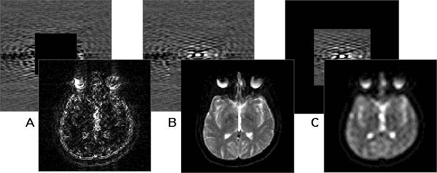 |
| Figure 6. Data acquired near the origin of k-space contains low spatial frequency information about the image, that acquired towards the k-space periphery represents high spatial frequencies. Figure B, above, shows the k-space raw data (from an EPI scan) and resulting image for a normal EPI scan. If the k-space data are zeroed, as in A, only the high spatial frequencies remain and the resulting image contains mostly thin lines. When only the low spatial frequency data are used, as in C, a low resolution image is produced. Note that the broad image contrast features are reasonably well represented in image C. Many strategies for increased conventional imaging speed, such as "Fast Spin Echo [6] " and "Keyhole Imaging [31] " take advantage of this in controlling image contrast. |
A few added notes about k-space (stated without proof):
The flow chart for true EPI (figure 7A) is much simpler than for conventional encoding (we will use the term "true EPI" to refer to scan techniques using a single excitation pulse), in that all data are acquired following a single excitation pulse, so that the signal need not be repeatedly re-formed. The key in this case, is to use higher gradient amplitudes and faster sampling (both requiring more advanced hardware) so that the total spatial encoding process is completed in a time short compared to T2, in other words, before the MR signal has decayed away. The path shown is for a particular k-space traversal known as MBEST [3] or Instascan [4], though others will be discussed below.
 |
| Figure 7A (top). Similar to the flow chart shown for conventional imaging in figure 4, in the scheme for the most common form of EPI, each line of data collection on the readout axis is separated by a brief pulse of the phase encoding gradient. The key, in true EPI, is to acquire each readout line fast enough that all can be acquired in the short time that the MR signal is present.
Figure 7B (bottom). The k-space trajectory for this form of EPI forms a raster-like path. Note that the direction of traversal for alternate lines of readout must be reversed by switching the polarity of the readout gradients. |
For completeness, we note that the so-called RARE [5] or Fast Spin Echo technique [6] is somewhere in the middle. In RARE, rather than use a new excitation pulse with each readout line, an additional 180° echo-forming pulse is used to re-form the signal. With RARE, the number of lines acquired per RF excitation may be easily increased (and the scan time correspondingly decreased) as much as sixteen-fold as compared to conventional imaging. Likewise, the GRASE technique [7] acquires a few readout lines following each of several RF spin echoes, finding a further spot in the middle ground between conventional and EPI approaches.
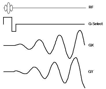
Having come up with the desired method of collecting the raw data, and given our simple knowledge of k-space, it is a relatively simple matter to write down the MR pulsing sequence needed for EPI. Figure 8 shows a straightforward version, using only a single excitation pulse. The RF pulse is made slice selective by simultaneously turning on a gradient along the slice selection axis. The Phase and Readout gradients (G-Phase and G-Readout, respectively) give the k-space trajectory of figure 5. Note that the positive-negative alternation of the readout gradient gives the alternating positive and negative velocities in k-readout, while the brief pulses, or "blips" [3] of the phase encoding gradient move the data from line to line along that axis.
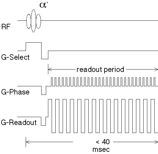 |
| Figure 8. Echo planar imaging pulse sequence used to create the k-space trajectory of figure 5. G-select, G-Phase and G-Readout refer to gradients on the slice selection, phase encoding and readout axes respectively. Excitation is limited to a single slice by transmitting the RF pulse in the presence of G-select. After that, brief negative pulses of G-Phase and G-Readout displace the signal to the lower left corner of k-space. Rapidly oscillating the readout gradient causes the signal trajectory to alternate in the positive and negative directions in the readout axis. The brief pulses or "blips" of G-Phase cause the trajectory to move up one line at a time along k-phase. A typical EPI scan time of 40 msec is shown to scale. |
Note the burden placed on the gradient system to perform such a sequence. For example, let's assume that we desire 2 mm pixels with a 0.5 msec readout period per line (a 32 msec readout for 64 phase encode lines). We more or less invert the discussion on resolution above and calculate that 2 mm resolution implies one cycle per 2 mm and that this must take place in 0.5 msec. The spins isochromats must therefore differ by 2 kHz in 2 mm or 10 kHz/cm which is a rather large gradient amplitude of (10 kHz /cm)/(4,258 Hz/gauss) or 2.35 gauss/cm. Furthermore this assumes that the gradients can be switched on to that value instantaneously, an unlikely feat.
All of the data points that make up the scan matrix along the readout axis must be acquired during the readout of each line. Thus, for a 128 point readout resolution, 128 points must be sampled during the gradient pulse. With readout periods of only 0.5 msec, the points must be sampled at 256 kHz, typically with 16 bits of precision, again assuming that the gradients have instantaneous rise times. This is quite close to today's (1995) practical limit for analog to digital conversion.
Just how many points need to actually be acquired depends upon the final image resolution and field of view needed. Where the maximum displacement along the k axis determines the image resolution, the FOV is determined by the number of points along that line, that is the number of data samples acquired between k=0 and kmax. For example, 128 pixels of 2 mm width will give a 25.6 cm FOV. Acquiring additional lines in the k-phase direction is easily done by simply extending the pulse sequence for a longer period. Unfortunately, this can result in some image distortion [8], as the T2*'s of the sample may not be long enough to yield signal for the extended readout duration. With today's imagers, matrix sizes of 128 lines (in the phase encode direction) are common, with readout periods as short as 60 msec.
As mentioned above, there is an important redundancy in the k-space raw data. The raw data can be decomposed into two components. One is symmetrical about the origin (like a cosine wave), and the other is anti-symmetric (like a sine wave). Knowing this, as long as one knows the precise location of that point of symmetry, it is possible to make a full image from only half of the data [1, 9] since the symmetrical and antisymmetrical parts of the data are easily constructed. Figure 9 shows the time evolution of the MR signal in the presence of gradients as the gradient-time integral approaches and passes through zero (k goes from negative to positive values). The magnetization of the sample is a rotating signal. If one imagines detecting the signal from two receivers rotated 90° with respect to one another, one would obtain the signals shown. One portion of the signal is symmetric about the k=0 point, and the other is anti-symmetric - its amplitude at time=-t is equal and opposite that at time=t. Clearly for waveforms of this kind, it would not be necessary to explicitly acquire the data at positive and negative k values.
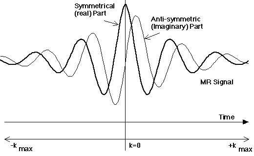 |
| Figure 9. The MR signal during gradient encoding. The MR signal is a rotating magnetic vector. Receivers 90° of rotation apart will detect the waveforms shown above, one of which is symmetric about k=0 and one of which is anti-symmetric. The technique of conjugate synthesis is frequently used in both conventional and echo-planar MR imaging to "synthesize" half of the data when the other half is explicitly collected. For example, if only the data in the positive portion of k-space were collected, it is a simple task to reconstruct the data for negative k-values. In practice, the symmetry is not perfect, due to such effects as T2 decay, motion and magnetic field inhomogeneity. It is usually therefor necessary to collect more than half of the data to form a satisfactory estimate of the other half. |
One way to understand this is the following. The Fourier transform, in general, operates between functions of complex variables. Even if the input function contains only real components, its transform generally contains an imaginary part, usually represented as a separate data set. Thus, for a single real input signal (from a real patient or phantom) two raw data sets are produced - real and imaginary. This implies that the transformed MR data are over-specified giving two transform points for every input point. This over specification is manifest as a symmetry in the MR raw data: if the value of the signal at k(m, n) is A + iB, the value at k(-m, n) will be A - iB, the complex conjugate. Knowing this, it is a trivial matter to calculate k(-m, n), if k(m, n) is known.
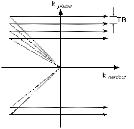
This so-called conjugate symmetry of the MR raw data for real objects affords a great savings in EPI and in conventional imaging, because only half of the raw data points need be acquired to form a complete image. Therefore, only half of the readout time is needed. In practice, however, determining the point of symmetry in the MR raw data requires collecting just slightly more than half of the data. Conjugate symmetry may be used in a variety of important ways in EPI, either to reduce the total scan time (relaxing somewhat the gradient requirements) or to improve the spatial resolution with a constant total readout. Let us suppose, for example, that we have a gradient set capable of achieving a desired FOV (say 20 x 40 cm) in a readout period of 32 msec, sweeping out the area of k-space shown in figure 10.
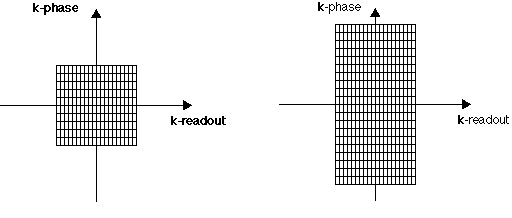 |
| Figure 10. During a single encoding cycle with EPI, a sufficient region of k-space is covered to produce a single image of moderate resolution, as indicated by the sampling grid above. Extending the overall readout duration (right) results in increased coverage of the k-phase axis, and thus improved resolution in that dimension. |
One important use of conjugate symmetry is in echo time reduction. Because the overall readout periods in EPI are rather long, the echo time (usually coincident with the collection of the central region of k-space) tends to be long as well. By explicitly collecting only half k-space, and starting near the origin, it is possible to dramatically reduce the effective TE. The data are then reconstructed by calculating the symmetrical half of the raw data space. Figure 11 outlines this scheme.
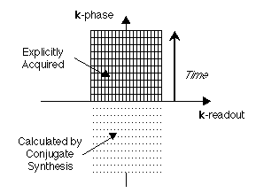 |
| Figure 11. Conjugate synthesis may be used for echo time reduction in EPI. The raw data are collected starting near the origin, closely following the RF excitation pulse and slightly more than half of k-space is covered. Conjugate symmetry is then exploited to complete the raw data set and a complete image is reconstructed. Using this approach, it is practical to achieve effective echo times of only a few milliseconds. |
It is also common to use conjugate synthesis to enhance spatial resolution. As suggested in figure 12, one can acquire data for a long readout period (as in figure 10, right) offset to one side of the k-readout axis. The other half of the raw data is then formed as before by conjugate synthesis. Using this approach, it is straightforward to acquire single shot images of 128x256 resolution, with pixel sizes of 1.5x3 mm.
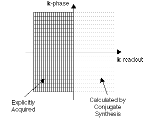 |
| Figure 12. The conjugate symmetry of k-space may be used for resolution-enhancement as shown above. Here, half of the data are explicitly collected along the k-readout axis, and the remaining half of the data are calculated. In combination with an extended readout duration as diagrammed in figure 11 (right), useful matrix sizes of 128 x 256 points may be collected in abut 60 milliseconds. |
Near the origin of k-space there is very little net spatial encoding, implying that these points represent the signal intensities of large areas in the image. As a result, these data points dominate the overall contrast features. Figure 6 (above) shows the contributions of the central and peripheral data points in k-space to the final image contrast.
For many applications, it is convenient to express the bandwidth of MR images as the frequency difference from one pixel to the next; this, in turn, is determined by the time that elapses between collection of adjacent pixels: with longer times resulting in lower effective bandwidths. The bandwidth is an extremely important parameter for the final image quality, as it determines the distortion in the final image from chemical shift and magnetic susceptibilities. Differences in susceptibility or chemical shift result in small differences in the proton resonant frequency. Since the positions of the signal are mapped onto the image by frequency, this can result in positional shifts and distortion. For typical conventional images, the frequency difference between pixels is generally set to about 125 Hertz. Fat and water have a relative chemical shift of about 3.5 parts per million (ppm), meaning that their resonant frequencies differ by 3.5 x 10-6 * 42.6 MHz/Tesla or about 150 Hz/Tesla. Thus, in a one Tesla field, fat and water would differ in position by about 1 pixel. In addition to the more familiar chemical shift, biological samples (such as people) typically exhibit susceptibility gradients on the order of 1-2 ppm between body tissues.
With the bandwidths used in conventional MRI, these susceptibility variations seldom exert much influence on the scans. In EPI, however, the effective bandwidth can be quite low, as the time between adjacent points on the k-phase axis can be quite long (0.5 to 1 msec) and there is no intervening RF pulse to rephase the MR signal. With a resulting bandwidth of 15 to 30 Hz/pixel, displacements of 8 to 10 pixels between water and fat, or in magnetically inhomogeneous regions such as the sella, are not uncommon. This problem is particularly serious in very high field imaging, as is being explored currently [10], because the frequency difference is proportional to the main magnetic field strength. As a consequence, the EPI readout must be faster at higher fields to maintain the same degree of image distortion.
Bandwidth is also related to signal to noise ratio. Lower image bandwidths incorporate less noise in the final images, as the higher frequencies are not sampled, and therefore high frequency noise does not contaminate the data set. The longer readout periods used for EPI at lower magnetic fields thus mitigate somewhat the reduction in signal strength in those instruments.
In the vast majority of applications, the EPI scans are acquired with lipid suppression to minimize the image degradation of prominent chemical shift artifacts. The most common scheme is to apply a saturating pulse to the fat resonance prior to data acquisition [11, 12], though other methods are viable. One promising approach is to use combined chemical shift and slice selective excitation (the so-called spatial-spectral pulse) [13], or short TI inversion recovery (STIR) [11, 14].
The raster-like k-space traversal shown above is only one of several that have been used for EPI. What is most important is that the raw data space be adequately covered by whatever traversal is used, regardless of the order in which the points are collected. One attractive approach is to cover the raw data space in a spiral pattern from the center of k-space outward (figure 13). Using this scheme, the echo time (defined as the time from the RF pulse to acquisition of the center of k-space) can be kept to an absolute minimum. (Note that the overall contrast behavior of the image is largely dominated by the data acquired at or near the center of k-space, as mentioned above.) Interestingly, the spiral acquisition pattern is self-refocusing for motion, so that velocity-dependent phase changes are minimized. This may become an advantage in vascular applications where velocities can be high even by comparison to the short overall readout used in EPI. Furthermore, the power requirements for the gradient sets are somewhat less severe, as the high amplitude gradient waveforms need not be reached instantaneously, as suggested in the raster EPI scheme described above.
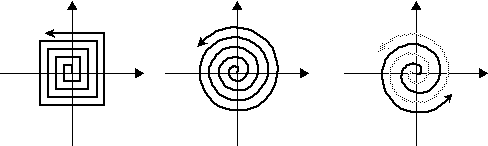 |
| Figure 13. As long as a sufficient number of points are acquired throughout the k-space plane it is possible to form a complete MR image. A variety of different traversal patterns have been proposed and used. The "square spiral" scan shown on the left has the advantage (as does the raster pattern shown in figure 7B above) that the data are acquired on a regular grid, so that a simple fast Fourier transform reconstructs the image. For the circular spiral and interleaved circular spiral trajectories on the middle and right, the gradient switching burden is minimized. |
The "square spiral" traversal shown in figure 13 on the left (as proposed and used by [15], like the MBEST/Instascan patterns in figure 7), has the advantage that the data are acquired on a regularly spaced grid. When acquired in this way, the data have only to be sorted before using a 2 dimensional Fourier transform for image reconstruction. When non-square (e.g. circular) spirals are used, as in figure 13 on the middle and right, the data cannot be acquired on such a grid. It therefore becomes necessary to adjust for the spacing of the data points, either by interpolation (which results in some loss of resolution and signal to noise ratio) or by non-Fourier reconstruction. On the other hand, the gradient switching cycle for the square spiral is extremely demanding. That for the circular spiral (figure 14) is much less so, being essentially a sinusoidal modulation of the form: Gx = ktsin(wt), Gy = ktcos(wt).
 |
| Figure 14. Gradient switching pattern required for the implementation of a circular spiral traversal of k-space, as sketched in figure 13. The gradient waveform can be drawn directly from the k-space traversal. Note that this is essentially a sinusoid of constantly increasing amplitude. |
The most challenging aspect of the spiral acquisitions, however, is the propagation of chemical shift and susceptibility artifacts. The raster scans of figure 7B result in the data along the phase (or frequency) encoding axis being sampled uniformly in time and therefore have a consistent effective bandwidth in either direction: chemical shift and susceptibility result in uniform positional shifts. In the spiral scans, the data points are sampled irregularly in time along these axes and thus result in blurring. The correction currently in practice for this problem is to reconstruct the raw data repeatedly at a variety of frequency offsets, and then to "focus" the image data from the various reconstructions [16]. This method is somewhat complex and computation-intensive, though nevertheless effective.
Errors in the amplitude of the gradient waveforms (or, more accurately, errors in positioning the sampling points with respect to the integral of the gradient) can result in improper location of the data points in k-space. The signal to noise ratio of single short EPI experiments can be surprisingly high, on the order of several hundred to one in head images at 1.5 Tesla when surface coils are used. Thus, such artifacts may frequently become visible. In order to use simple Fourier methods to reconstruct the EPI scans, it is desirable that the data points be spaced on a regular 2 dimensional grid. As suggested in figure 3, this may be accomplished either by sampling at a constant rate in the presence of a constant gradient amplitude, or by sampling at an irregular rate in the presence of a non-constant gradient, as long as the integral of the gradient, with respect to time, is kept constant between successive data points. Many current practical implementations of gradient power systems utilize sinusoidal gradient waveforms as they can be made quite power efficient through the use of resonant controllers [17]. Such an approach to sampling requires high resolution in the sampling control system, as small timing errors in each data point may result in noticeable artifacts.
The most common, and ultimately most challenging, source of such sampling errors is through the introduction of magnetic eddy currents in the conducting surfaces of the magnet, due to the relatively high switching fields from the gradients. Such eddy currents result in time-dependent distortions of the magnetic field and thus in variations in the precessional frequency of the protons. The spatial distribution of the eddy current fields depend upon their conduction paths; in some cases they may result primarily in an overall field shift (when, for example, the conducting path forms a loop around the magnet's imaging bore) or in gradient fields. Either of these will introduce distortion into the spatial encoding of the signal.
Eddy currents in EPI are so serious that in practice some sort of gradient shielding is generally required (unless local gradient coils that are at a considerable distance from the conducting surfaces of the magnet are used). The most commonly used approach to gradient shielding is to use a concentric, counter-wound gradient set that cancels the gradient fields outside of the coil [18]. Of course, this also attenuates the gradients on the inside of the coil so that the overall efficiency of the gradient may be reduced.
The timing of the samples must also be quite accurate to minimize artifacts. Collecting 256 data samples during a 500 µsec gradient pulse requires sampling at an average of 500 kHz. In most practical applications of EPI, the actual sampling rate is much higher, as the gradient waveshape is sinusoidal or trapezoidal (rather than square). Since the gradient is not on at full strength for the entire 500 µsec readout, the peak amplitudes, and thus sampling rate must be higher. Roughly speaking, the amplitude of the artifacts increases linearly with the errors in sampling rate. Thus, to keep such artifacts below the 200:1 SNR, the sampling must be accurate to within 0.5 parts per hundred, or 1 x 10⁻⁸ seconds with the 2 µsec samples described above.
One common form of sampling error is for the entire sampling train to be offset by a few microseconds from the gradient waveform. This can happen, when, for example, slight phase lags appear in the RF receiver system due to variations in the RF coil characteristics. Because the data in ordinary EPI are acquired in a back and forth trajectory in k-space, alternate data lines must be reversed in time prior to Fourier reconstruction. A small lag in the sampling therefore results in a line to line k-space discrepancy, with alternate lines being properly phased. This will result in the introduction of ghost artifacts into the image, as schematized in figure 15.
 |
| Figure 15. So-called "N/2" ghost artifact that appears when alternating lines of k-space are not sampled in proper phase coherence, as can happen when sampling time points are shifted slightly with respect to gradient switching. |
In much the same way that individual raw data lines may be concatenated across excitations to form a complete conventional image, it is reasonable, and practical to concatenate one or more EPI data acquisitions traversing different regions of k-space to form a higher resolution image. This is the principal behind both the "Mosaic" and "MESH" methods proposed by Rzedzian [14, 19]. In the Mosaic scan, 2D tiles of k-space data are acquired and concatenated prior to image reconstruction. In the MESH scans, the EPI data collections are interleaved along the phase encoding axis.
Another multiple excitation ("multi-shot") EPI approach is to provide phase-encoding along the slice selection axis between each EPI data collection. A 3D Fourier transform of this data set results in a multi-slice, volume data set [20]. Because each of the resulting images is formed from the entire data set a net improvement in signal to noise ratio is achieved. As a result it is possible to form very high resolution contiguous data sets in an extremely short period. Cohen, for example, has demonstrated 4 mm contiguous sections of the heart in total scan times of only 400 msec [21], easily fast enough to minimize artifacts from cardiac motion. Volume acquisitions, however, place a significant burden on the analog to digital conversion system in the scanner, as achieving the predicted high signal to noise ratio requires high digitization depth (on the order of 16 bits) while maintaining the high EPI sampling rate. Fortunately, this is now becoming economically feasible.
As shown by Ampére, time varying magnetic fields (dB/dt) results in the development of an electromotive force and thus a current in nearby conductors. The switching rate of gradients used in EPI systems can readily reach amplitudes of more than 100 Tesla/second that can produce significant electrical currents in the body of the subject being imaged [22-25] that can, under certain circumstances, be perceived and can even become quite noxious. The current magnitude depends on such factors as the orientation of the time-varying fields with respect to the conducting paths of the body, the local electrical conductivity, etc. The sensory effects depend, in addition, on the direction of the nerve fiber bundles with respect to the induced electric fields. In humans, in body gradient sets, the threshold for delectability of the gradients seems to be about 60 T/sec r.m.s. with gradients operating near 1 kHz [25, 26]. On theoretical grounds, usage of trapezoidal as opposed to sinusoidal, gradient waveforms may results in slightly greater total gradient areas, and thus higher spatial resolution, before stimulation can be detected [27, 28]. Safety of the EPI system is therefore of significant concern to both the system designers and to regulatory agencies.
The available evidence on safety is presently very limited, as there are no reports of practical imaging designs that are able to cross safety thresholds. One group has studied the effects of extremely high magnetic field switching rates (3000 Tesla/second) applied locally to the myocardium of laboratory animals. At these dB/dt's they were able to produce extra-systoles [29]. Such data suggest a considerable safety margin between the detection of gradient induced currents in the body and their possible harmful effects. Prudent gradient designs, however, ordinarily minimize the dB/dt where possible.
It is sometimes convenient to consider EPI as a sort of stand-alone imaging block in a pulse sequence, where the RF pulse sequence determines the image contrast and an EPI encoding step forms an image from the MR signal at any time point. For example, performing EPI spatial encoding following a single excitation pulse results in an image whose contrast is T2* dominated (i.e. its signal intensity depends strongly on local magnetic field variations). Using a two pulse series, typically a 90° pulse followed by a 180° pulse (a Hahn spin echo series [30] ), with a subsequent EPI data collection resulting in an image where the T2* contrast is minimized. Compared to conventional imaging, the typical readout period of 30 to 128 milliseconds in EPI is rather long, and T2* losses are considerable during the readout period. Hahn echoes are commonly required for reasonable image quality.
As practiced at the time of this writing, EPI is a rapidly emerging approach to MR imaging. Compared to conventional scanning it offers tremendous speed advantages (of several hundred fold for comparable contrast) and a greatly expanded range of applications. Because the sampling duration is considerably shorter, the SNR may be limited - therefore EPI is predominantly a high field (1.5 Tesla, or more) technique. The engineering difficulties in high speed, high amplitude gradient and analog to digital conversion designs have been largely overcome, so that readout gradient oscillation rates of 800 Hz to 1400 Hz are now practical, enabling 256 x 256 images to be collected in as little as 90 msec (using conjugate synthesis). EPI imaging speed is thus facing other practical limits, such as the threshold of sensation from the large dB/dt and the SNR loss that can result from extremely short readouts (and large bandwidths). The gradient hardware, in particular, remains quite costly. EPI is therefore not yet widely available but costs are showing a definite trend downward. The ultimate acceptance of EPI will depend now primarily on the value of the new applications as compared to the cost of the technology conversions.